Revenue theory (HL only)

Introduction

This lesson focuses on more definitions of costs and revenue and contains several paper three-type questions. Learning by doing is an effective way for your students to learn the primary concepts.

Inquiry question

Understanding the terms total revenue, average revenue, and marginal revenue

Teacher notes

Lesson time: 55 minutes

Lesson objectives:

Distinguish between total revenue, average revenue, and marginal revenue.

Draw diagrams illustrating the relationship between total revenue, average revenue, and marginal revenue.

Calculate total revenue, average revenue, and marginal revenue from a set of data and/or diagrams.

Teacher notes:

1. Beginning activity - begin with the opening activity and allow 5 minutes for discussion. I like to ask students to give me a definition of the two terms as a way of starting the lesson off. You may also wish to quickly differentiate between the terms total revenue and sales revenue. (10 minutes)

2. Processes - technical Vocabulary - the students can learn the key concepts through the notes, which should take ten minutes to go through and discuss. (10 minutes)

3. Practise activities included on the handout should take around 30 minutes.

4. Final reflection exercise - considers the difference between a firm's revenue and profit maximising output levels.

Beginning question

What is meant by the term revenue? What is the difference between revenue and profit?

While some IB students confuse the two terms, revenue refers to monies coming into the business, while profit is calculated by revenue minus the costs of the business, including implicit costs.

Key terms:

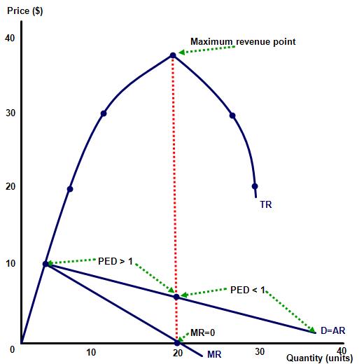
Total revenue (TR) is the total revenue produced by a firm, measured in monetary terms usually in $. This is also sometimes called sales revenue. It is calculated by selling price or average revenue multiplied by output.

Marginal revenue (MR) is the additional revenue generated when one good or service is added. As the output is increased the MR will fall sharply as the supply of the product has risen. In economics, we presume that as a good becomes less scarce its price will fall. MR is calculated by the formulae Δ TR / Δ Q.

Average revenue (AR) is the average revenue produced per unit of output. Like MR, average revenue also falls as output rises but does so at exactly half the rate of decline of MR i.e. the downward slope of the AR curve falls at half the gradient of the MR curve.

The activities on this page can be downloaded as a PDF file at Revenue theory

Activity 1

(a) A firm is looking to increase its sales revenue and is producing a PED elastic good. What course of action should the business take?

Using a simple law of economics the business can increase its revenue by lowering the price of the good or service, as they gain in revenue from additional sales will more than compensate for the lower unit selling price.

(b) A firm is looking to increase its sales revenue and is producing a PED inelastic good. What course of action should the business take?

Again using the same simple law this business can raise revenue by doing the opposite, raising the price of the product, as the gain in revenue from the higher selling price will more than compensate for the lower than proportional fall in quantity demanded.

(c) If a theoretical business was producing a perfectly elastic good (PED = infinity) then explain what will happen to both MR and AR as the firm raises its output?

As the question states this is a theoretical concept only but in this instance both MR and AR would remain unchanged. This is because with the business being very small, compared to the total market, the firm can raise their output without impacting on market supply and hence selling price.

Activity 2

(a) Complete the following table by adding the missing blanks:

Selling price $ (AR)	Number of workers required quantity quantity	Quantity sold	Total revenue ($)	Marginal revenue ($)	Price elasticity of demand (PED)
10	1	2	20		(%Δ in Q) = 100 / (10 = (%Δ in P)
				8 (Δ in TR) / (Δ in Q) i.e 16/2
9	2	4	36		4.55
				6
8	3	6	48		2.64
				4
7	4	8	56		1.75
				2
6	5	10	60		1.2
				0
5	6	12	60		0.84
				(2)
4	7	14	56		0.52
				(4)
3	8	16	48		0.38
				(6)
2	9	18	36		0.22
				(8)
1	10	20	20		0.1

Activity 3

Complete the table by filling in the missing blanks in the table:

Selling price (AR) $	Number of workers required quantity quantity quantity	Quantity sold	Total revenue ($)	Marginal revenue ($)	Price elasticity of demand (PED)
150	5	10	1,500		(%Δ in Q) = 50 / 6.67 (%Δ in P) = 7.50
				(Δ in TR) / (Δ in Q) i.e 600/5 = $120
140	6	15	2,100		(%Δ in Q) = 33.33 / 7.14 (%Δ in P) = 4.67
				$ 100
130	7	20	2,600		(%Δ in Q) = 25 / 7.69 (%Δ in P) = 3.25
				$ 80
120	8	25	3,000		(%Δ in Q) = 20 / 8.33 (%Δ in P) = 2.40
				$ 60
110	9	30	3,300		(%Δ in Q) = 16.66 / 9.09 (%Δ in P) = 1.83
				$ 40
100	10	35	3,500		(%Δ in Q) = 14.28 / 10 (%Δ in P) = 1.43
				$ 20
90	11	40	3,600		(%Δ in Q) = 12.5 / 11.11 (%Δ in P) = 1.26
				0
80	12	45	3,600		(%Δ in Q) = 11.11 / 12.5 (%Δ in P) = 7.42 = 0.89
				($ 20)
70	13	50	3,500		(%Δ in Q) = 10 / 14.29 (%Δ in P) = 0.70
				($ 40)
60	14	55	3,300		(%Δ in Q) = 9.09 / 16.67 (%Δ in P) = 0.55
				($ 60)
50	15	60	3,000		-

Draw on a piece of graph paper the MR and AR curves.

Hint when plotting the above information

If you have drawn your graphs properly using the correct scales then your MR curve should fall at twice the gradient of the average revenue. In addition, while your marginal revenue curve will fall below zero the AR should not do so.

Activity 4

(a) Complete the following table:

Output level	Total revenue $ (000)	Total cost $ (000)	MR	MC	Total profit $ (000)
100	350	300			50
			(Δ in TR) / (Δ in Q) i.e 200/100 = $2,000	(Δ in TC) / (Δ in Q) i.e 60,000/100 = 600
200	550	360			190
			1,600	800
300	710	440			270
			1,200	900
400	830	530			300
			1,000	1,000
500	930	630			300
			800	1,050
600	1,010	735			275
			700	1,100
700	1,080	845			235
			600	1,120
800	1,140	957			183
			0	1,150
900	1,140	1,072			68
			(20)	1,990
1,000	1,120	1,271			(151)

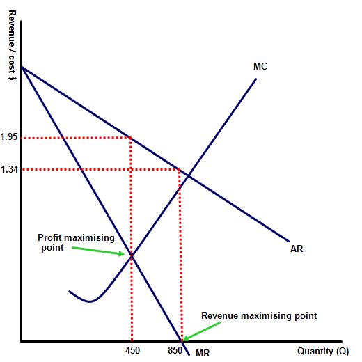
(b) Illustrate the level of output at the profit maximising point

Activity 5: Reflection

Why are the profit maximising and revenue maximising levels of output different? Shouldn't profit also be maximised where revenue is at its highest.

Surprisingly no, revenue is maximised at where MR=0 whereas firms will often produce below this level to drive up the price and maximise their profit level at where MC=MR.

IBDP Economics - Student pages

INTHINKING REVISION SITES

www.StudyIB.net