 IB Docs (2) Team

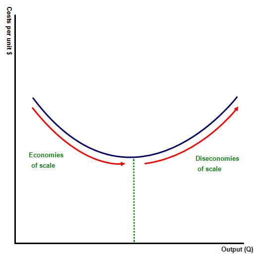
Long run average cost curves (HL only)
 Introduction
This page simply looks at the concept of the long run in economics and considers why businesses experience firstly economies of scale and then diseconomies of scale as they increases output levels.
Enquiry question
Classifying different costs of production in the long run.
 Teacher notes
Lesson time: 45 minutes
Lesson objectives:
Explain the relationship between short-run average costs and long-run average costs.
Explain, using a diagram, the reason for the shape of the long-run average total cost curve..
Teacher notes:
1. Beginning activity - begin with the opening video and allow 10 minutes for discussion
2. Processes - technical Vocabulary - the students can learn the key concepts through the activities provided. (30 minutes)
3. Final reflective activity - Project the paper one type question on to the whiteboard so that your classes can reflect on it. Have them answer this question in their notebooks or even complete the question as a homework exercise. (5 minutes)
Key term:
LRAC curve - consists of a locus of points, each representing the most efficient level of production in the short run.
Economies of scale - a firm experiences economies of scale when they are experiencing increasing returns to scale. This includes any processes which enable a firm to reduce its long run average costs as output rises.
Internal economies of scale - economies arising from any economy or benefit which comes from inside the company and are usually associated with increased specialisation in the way that the business operates.
The activities on this page are available as a worksheet at: ![]() LRAC
LRAC
Beginning activity
Watch the following short video and then answer the questions which follow:
(a) Does the planning process exist in the short run or the long run?
Long run
(b) In the short run the firm can only change which type of costs?
Variable costs
(c) Draw a long run average cost curve showing both economies and diseconomies of scale.
Activity 2
You start a business producing hand made greetings cards with your friends. You think you have all bases covered - you are a talented IB visual arts student and your friends study business management and economics. You feel confident in your new business. You set up in your spare bedroom and you initially make your cards by hand. Due to high demand, however, you soon have to increase output and this means purchasing a printing machine. As demand for your product rises you hire additional workers to help with the workload as well as extra printing machines to satisfy demand for your product. The following table illustrates the range of inputs and outputs for the business in an average day.
| Number of workers | Number of machines | Output | Production cost $ | Average cost $ |
| 1 | 0 | 10 | 33 | 3.30 |
| 2 | 0 | 20 | 64 | 3.20 |
| 3 | 0 | 30 | 93 | 3.10 |
| 1 | 1 | 40 | 120 | 3.00 |
| 2 | 1 | 50 | 145 | 2.90 |
| 3 | 1 | 60 | 168 | 2.80 |
| 3 | 2 | 70 | 189 | 2.70 |
| 4 | 2 | 80 | 224 | 2.80 |
| 5 | 2 | 90 | 261 | 2.90 |
| 5 | 3 | 100 | 300 | 3.00 |
| 6 | 3 | 110 | 341 | 3.10 |
| 7 | 3 | 120 | 384 | 3.20 |
| 8 | 3 | 130 | 429 | 3.30 |
Questions
a. Using a piece of graph paper plot the above average cost curve for the information in the table. The vertical axis should be labelled average cost and the horizontal axis output.
b. Why do average costs initially fall before rising?
Initially as the firm increases inputs of labour and machinery output rises as the new workers add to the production process. Initially two workers can produce twice as much as one e.t.c. and perhaps even more if they can make full use of greater specialisation. Also as more machines are purchased output rises. As output rises quickly average costs will fall as the level of output rises at a faster rate than the rise in number of inputs (labour, machinery and materials). This is called increasing returns to scale. However as the rate of increase in output declines the output per worker falls, leading to higher average costs. This is called diseconomies of scale.
Activity 3
Complete the following table by adding in the missing values:
Units produced | Total cost (TC) | Average cost (AC) | Marginal cost (MC) | Average fixed cost (AFC) | Average variable cost(AVC) |
0 | 10 | - | - | - | |
5 | |||||
10 | 60 | 6 | 1 | 5 | |
4 | |||||
20 | 100 | 5 | 0.5 | 4.5 | |
2 | |||||
30 | 120 | 4 | 0.33 | 3.67 | |
2 | |||||
40 | 140 | 3.5 | 0.25 | 3.25 | |
3.5 | |||||
50 | 175 | 3.5 | 0.2 | 3.3 | |
6.5 | |||||
60 | 240 | 4 | 0.17 | 3.83 | |
11 | |||||
70 | 350 | 5 | 0.14 | 4.86 | |
13 | |||||
80 | 480 | 6 | 0.13 | 5.88 |
Note that in Paper 3 HL, students may be asked to calculate the above figures from the information provided.
 Twitter
 Facebook
 LinkedIn