HL Paper 3
The weights, X kg, of the males of a species of bird may be assumed to be normally distributed with mean 4.8 kg and standard deviation 0.2 kg.
The weights, Y kg, of female birds of the same species may be assumed to be normally distributed with mean 2.7 kg and standard deviation 0.15 kg.
Find the probability that a randomly chosen male bird weighs between 4.75 kg and 4.85 kg.
Find the probability that the weight of a randomly chosen male bird is more than twice the weight of a randomly chosen female bird.
Two randomly chosen male birds and three randomly chosen female birds are placed on a weighing machine that has a weight limit of 18 kg. Find the probability that the total weight of these five birds is greater than the weight limit.
Markscheme
Note: In question 1, accept answers that round correctly to 2 significant figures.
P(4.75 < X < 4.85) = 0.197 A1
[1 mark]
Note: In question 1, accept answers that round correctly to 2 significant figures.
consider the random variable X − 2Y (M1)
E(X − 2Y) = − 0.6 (A1)
Var(X − 2Y) = Var(X) + 4Var(Y) (M1)
= 0.13 (A1)
X − 2Y ∼ N(−0.6, 0.13)
P(X − 2Y > 0) (M1)
= 0.0480 A1
[6 marks]
Note: In question 1, accept answers that round correctly to 2 significant figures.
let W = X1 + X2 + Y1 + Y2 + Y3 be the total weight
E(W) = 17.7 (A1)
Var(W) = 2Var(X) + 3Var(Y) = 0.1475 (M1)(A1)
W ∼ N(17.7, 0.1475)
P(W > 18) = 0.217 A1
[4 marks]
Examiners report
The random variables \(U,{\text{ }}V\) follow a bivariate normal distribution with product moment correlation coefficient \(\rho \).
A random sample of 12 observations on U, V is obtained to determine whether there is a correlation between U and V. The sample product moment correlation coefficient is denoted by r. A test to determine whether or not U, V are independent is carried out at the 1% level of significance.
State suitable hypotheses to investigate whether or not \(U\), \(V\) are independent.
Find the least value of \(|r|\) for which the test concludes that \(\rho \ne 0\).
Markscheme
\({{\text{H}}_0}:\rho = 0;{\text{ }}{{\text{H}}_1}:\rho \ne 0\) A1A1
[2 marks]
\(\nu = 10\) (A1)
\({t_{0.005}} = 3.16927 \ldots \) (M1)(A1)
we reject \({{\text{H}}_0}:\rho = 0\) if \(\left| t \right| > 3.16927 \ldots \) (R1)
attempting to solve \(\left| r \right|\sqrt {\frac{{10}}{{1 - {r^2}}}} > 3.16927 \ldots \) for \(\left| r \right|\) M1
Note: Allow = instead of >.
(least value of \(\left| r \right|\) is) 0.708 (3 sf) A1
Note: Award A1M1A0R1M1A0 to candidates who use a one-tailed test. Award A0M1A0R1M1A0 to candidates who use an incorrect number of degrees of freedom or both a one-tailed test and incorrect degrees of freedom.
Note: Possible errors are
10 DF 1-tail, \(t = 2.763 \ldots \), least value \( = \) 0.658
11 DF 2-tail, \(t = 3.105 \ldots \), least value \( = \) 0.684
11 DF 1-tail, \(t = 2.718 \ldots \), least value \( = \) 0.634.
[6 marks]
Examiners report
A biased cubical die has its faces labelled \(1,{\rm{ }}2,{\rm{ }}3,{\rm{ }}4,{\rm{ }}5\) and \(6\). The probability of rolling a \(6\) is \(p\), with equal probabilities for the other scores.
The die is rolled once, and the score \({X_1}\) is noted.
(i) Find \({\text{E}}({X_1})\).
(ii) Hence obtain an unbiased estimator for \(p\).
The die is rolled a second time, and the score \({X_2}\) is noted.
(i) Show that \(k({X_1} - 3) + \left( {\frac{1}{3} - k} \right)({X_2} - 3)\) is also an unbiased estimator for \(p\) for all values of \(k \in \mathbb{R}\).
(ii) Find the value for \(k\), which maximizes the efficiency of this estimator.
Markscheme
let \(X\) denote the score on the die
(i) \({\text{P}}(X = x) = \left\{ {\begin{array}{*{20}{c}} {\frac{{1 - p}}{5},}&{x = 1,{\text{ 2}},{\text{ 3}},{\text{ 4}},{\text{ 5}}} \\ {p,}&{x = 6} \end{array}} \right.\) (M1)
\(E({X_1}) = (1 + 2 + 3 + 4 + 5)\frac{{1 - p}}{5} + 6p\) M1
\( = 3 + 3p\) A1
(ii) so an unbiased estimator for \(p\) would be \(\frac{{{X_1} - 3}}{3}\) A1
[4 marks]
(i) \(E\left( {k({X_1} - 3) + \left( {\frac{1}{3} - k} \right)({X_2} - 3)} \right)\) M1
\( = kE({X_1} - 3) + \left( {\frac{1}{3} - k} \right)E({X_2} - 3)\) M1
\( = k(3p) + \left( {\frac{1}{3} - k} \right)(3p)\) A1
any correct expression involving just \(k\) and \(p\)
\( = p\) AG
hence \(k({X_1} - 3) + \left( {\frac{1}{3} - k} \right)({X_2} - 3)\) is an unbiased estimator of \(p\)
(ii) \({\text{Var}}\left( {k({X_1} - 3) + \left( {\frac{1}{3} - k} \right)({X_2} - 3)} \right)\) M1
\( = {k^2}{\text{Var}}({X_1} - 3) + {\left( {\frac{1}{3} - k} \right)^2}{\text{Var}}({X_2} - 3)\) A1
\( = \left( {{k^2} + {{\left( {\frac{1}{3} - k} \right)}^2}} \right){\sigma ^2}\) (where \({\sigma ^2}\) denotes \({\text{Var}}(X)\))
valid attempt to minimise the variance M1
\(k = \frac{1}{6}\) A1
Note: Accept an argument which states that the most efficient estimator is the one having equal coefficients of \({X_1}\) and \({X_2}\).
[7 marks]
Total [11 marks]
Examiners report
It is known that the standard deviation of the heights of men in a certain country is \(15.0\) cm.
One hundred men from that country, selected at random, had their heights measured.
The mean of this sample was \(185\) cm. Calculate a \(95\% \) confidence interval for the mean height of the population.
A second random sample of size \(n\) is taken from the same population. Find the minimum value of \(n\) needed for the width of a \(95\% \) confidence interval to be less than \(3\) cm.
Markscheme
valid attempt to use \(\bar x \pm z\frac{\sigma }{{\sqrt n }}\) (M1)
\([182,{\text{ }}188]\) A1A1
Note: Accept answers that round to the correct \(3\) sf.
[3 marks]
\(1.96 \times \frac{{15.0}}{{\sqrt n }} < 1.5\) M1A1
\(n > {\left( {\frac{{15.0}}{{1.5}} \times 1.96} \right)^2}\) (M1)
Note: Award M1 for attempting to solve the inequality.
Note: Allow the use of \( = \).
minimum value \(n = 385\) A1
[4 marks]
Total [7 marks]
Examiners report
The strength of beams compared against the moisture content of the beam is indicated in the following table. You should assume that strength and moisture content are each normally distributed.
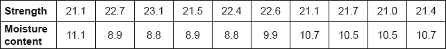
Determine the product moment correlation coefficient for these data.
Perform a two-tailed test, at the \(5\% \) level of significance, of the hypothesis that strength is independent of moisture content.
If the moisture content of a beam is found to be \(9.5\), use the appropriate regression line to estimate the strength of the beam.
Markscheme
\(r = - 0.762\) (M1)A1
Note: Accept answers that round to \( - 0.76\).
[2 marks]
\({H_0}:\) Moisture content and strength are independent or \(\rho = 0\)
\({H_1}:\) Moisture content and strength are not independent or \(\rho \ne 0\) A1
EITHER
test statistic is \(-3.33\) A1
critical value is \(( \pm ){\text{ }}2.306\) A1
since \( - 3.33 < - 2.306\) or \(3.33 > 2.306\), R1
reject \({H_0}\;\;\;\)(or equivalent) A1
OR
\(p\)-value is \(0.0104\) A2
as \(0.0104 < 0.05\), R1
reject \({H_0}\;\;\;\)(or equivalent) A1
Note: The R1 and A1 can be awarded as follow through from their test statistic or \(p\)-value.
[5 marks]
\(x = {\text{strength}}\)
\(y = {\text{moisture content}}\)
\(x = - 0.629y + 28.1\) (M1)(A1)
if \(y = 9.5\) so \(x = 22.1\) (M1)A1
Note: Only accept answers that round to \(22.1\).
Note: Award M1A1M0A0 for the other regression line \(y = 30.1 - 0.924x\).
[4 marks]
Total [11 marks]
Examiners report
Anna cycles to her new school. She records the times taken for the first ten days with the following results (in minutes).
12.4 13.7 12.5 13.4 13.8 12.3 14.0 12.8 12.6 13.5
Assume that these times are a random sample from the \({\text{N}}(\mu ,{\text{ }}{\sigma ^2})\) distribution.
(a) Determine unbiased estimates for \(\mu \) and \({\sigma ^2}\).
(b) Calculate a 95 % confidence interval for \(\mu \).
(c) Before Anna calculated the confidence interval she thought that the value of \(\mu \) would be 12.5. In order to check this, she sets up the null hypothesis \({{\text{H}}_0}:\mu = 12.5\).
(i) Use the above data to calculate the value of an appropriate test statistic. Find the corresponding p-value using a two-tailed test.
(ii) Interpret your p-value at the 1 % level of significance, justifying your conclusion.
Markscheme
(a) estimate of \(\mu = 13.1\) A1
estimate of \({\sigma ^2} = 0.416\) A1
[2 marks]
(b) using a GDC (or otherwise), the 95% confidence interval is (M1)
[12.6, 13.6] A1A1
Note: Accept open or closed intervals.
[3 marks]
(c) (i) \(t = \frac{{13.1 - 12.5}}{{0.6446 \ldots /\sqrt {10} }} = 2.94\) (M1)A1
\(v = 9\) (A1)
p-value \( = 2 \times {\text{P}}(T > 2.9433 \ldots )\) (M1)
\( = 0.0164\,\,\,\,\,\)(accept 0.0165) A1
(ii) we accept the null hypothesis (the mean travel time is 12.5 minutes) A1
because 0.0164 (or 0.0165) > 0.01 R1
Note: Allow follow through on their p-value.
[7 marks]
Total [12 marks]
Examiners report
This was well answered by many candidates. In (a), some candidates chose the wrong standard deviation from their calculator and often failed to square their result to obtain the unbiased variance estimate. Candidates should realise that it is the smaller of the two values (ie the one obtained by dividing by (n – 1)) that is required. The most common error was to use the normal distribution instead of the t-distribution. The signpost towards the t-distribution is the fact that the variance had to be estimated in (a). Accuracy penalties were often given for failure to round the confidence limits, the t-statistic or the p-value to three significant figures.
The random variable X has a geometric distribution with parameter p .
Show that \({\text{P}}(X \leqslant n) = 1 - {(1 - p)^n},{\text{ }}n \in {\mathbb{Z}^ + }\) .
Deduce an expression for \({\text{P}}(m < X \leqslant n)\,,{\text{ }}m\,,{\text{ }}n \in {\mathbb{Z}^ + }\) and m < n .
Given that p = 0.2, find the least value of n for which \({\text{P}}(1 < X \leqslant n) > 0.5\,,{\text{ }}n \in {\mathbb{Z}^ + }\) .
Markscheme
\({\text{P}}(X \leqslant n) = \sum\limits_{{\text{i}} = 1}^n {{\text{P}}(X = {\text{i}}) = \sum\limits_{{\text{i}} = 1}^n {p{q^{{\text{i}} - 1}}} } \) M1A1
\( = p\frac{{1 - {q^n}}}{{1 - q}}\) A1
\( = 1 - {(1 - p)^n}\) AG
[3 marks]
\({(1 - p)^m} - {(1 - p)^n}\) A1
[1 mark]
attempt to solve \(0.8 - {(0.8)^n} > 0.5\) M1
obtain n = 6 A1
[2 marks]
Examiners report
In part (a) some candidates thought that the geometric distribution was continuous, so attempted to integrate the pdf! Others, less seriously, got the end points of the summation wrong.
In part (b) It was very disappointing that may candidates, who got an incorrect answer to part (a), persisted with their incorrect answer into this part.
In this question you may assume that these data are a random sample from a bivariate normal distribution, with population product moment correlation coefficient \(\rho \).
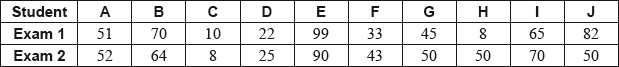
Richard wishes to do some research on two types of exams which are taken by a large number of students. He takes a random sample of the results of 10 students, which are shown in the following table.
Using these data, it is decided to test, at the 1% level, the null hypothesis \({H_0}:\rho = 0\) against the alternative hypothesis \({H_1}:\rho > 0\).
Richard decides to take the exams himself. He scored 11 on Exam 1 but his result on Exam 2 was lost.
Caroline believes that the population mean mark on Exam 2 is 6 marks higher than the population mean mark on Exam 1. Using the original data from the 10 students, it is decided to test, at the 5% level, this hypothesis against the alternative hypothesis that the mean of the differences, \({\text{d}} = {\text{exam 2 mark }} - {\text{ exam 1 mark}}\), is less than 6 marks.
For these data find the product moment correlation coefficient, \(r\).
(i) State the distribution of the test statistic (including any parameters).
(ii) Find the \(p\)-value for the test.
(iii) State the conclusion, in the context of the question, with the word “correlation” in your answer. Justify your answer.
Using a suitable regression line, find an estimate for his score on Exam 2, giving your answer to the nearest integer.
(i) State the distribution of your test statistic (including any parameters).
(ii) Find the \(p\)-value.
(iii) State the conclusion, justifying the answer.
Markscheme
\(r = 0.804\) A2
Note: Accept any number that rounds to 0.80.
[2 marks]
(i) \(t\) distribution with 8 degrees of freedom A1A1
(ii) \(p{\text{ - value}} = 0.00254\) A2
Notes: Accept any number that rounds to 0.0025.
Award A1 for 2-tail test giving an answer that rounds to 0.0051.
(iii) \(p{\text{ - value}} < 0.01\), so conclude that there is positive correlation R1A1
Notes: Only award the A1 if the R1 is awarded.
Do not accept just “reject \({H_0}\)” or “accept \({H_1}\)”.
The words “positive correlation” must be seen.
[6 marks]
regression line of \(y\) (Exam 2 mark) on \(x\) (Exam 1 mark) is (M1)
\(y = 0.59407 \ldots x + 21.387 \ldots \) (A1)
\(x = 11\) gives \(y = 28\) (to nearest integer) A1
[3 marks]
(i) applying the \(t\) test to the differences
\(t\) distribution with 9 degrees of freedom A1A1
(ii) \(p{\text{ - value}} = 0.239\) A2
Notes: Accept any number that rounds to 0.24.
Award A1 if subtraction done the wrong way round giving \(p{\text{ - value}} = 0.109\).
(iii) \(p{\text{ - value}} > 0.05\), so accept \({H_0}\) or \({u_d} = 6\) R1A1
[6 marks]
Examiners report
A random variable \(X\) is distributed with mean \(\mu \) and variance \({\sigma ^2}\). Two independent random samples of sizes \({n_1}\) and \({n_2}\) are taken from the distribution of \(X\). The sample means are \({\bar X_1}\) and \({\bar X_2}\) respectively.
Show that \(U = a{\bar X_1} + (1 - a){\bar X_2},{\text{ }}a \in \mathbb{R}\), is an unbiased estimator of \(\mu \).
Show that \({\text{Var}}(U) = {a^2}\frac{{{\sigma ^2}}}{{{n_1}}} + {(1 - a)^2}\frac{{{\sigma ^2}}}{{{n_2}}}\).
Find, in terms of \({n_1}\) and \({n_2}\), an expression for \(a\) which gives the most efficient estimator of this form.
Hence find an expression for the most efficient estimator and interpret the result.
Markscheme
\({\text{E}}(U) = E(a{\bar X_1} + (1 - a){\bar X_2}) = a{\text{E}}({\bar X_1}) + (1 - a){\text{E}}({\bar X_2})\) (M1)
\({\text{E}}({\bar X_1}) = \mu \) and \({\text{E}}({\bar X_2}) = \mu \)
\({\text{E}}(U) = a\mu + (1 - a)\mu \) (or equivalent) A1
\( = \mu \) A1
hence \(U\) is an unbiased estimator of \(\mu \) AG
[3 marks]
\({\text{Var}}(U) = {\text{Var}}(a{\bar X_1} + (1 - a){\bar X_2})\)
\( = {a^2}{\text{Var}}({\bar X_1}) + {(1 - a)^2}{\text{Var}}({\bar X_2})\) M1
stating that \({\text{Var}}({\bar X_1}) = \frac{{{\sigma ^2}}}{{{n_1}}}\) and \({\text{Var}}({\bar X_2}) = \frac{{{\sigma ^2}}}{{{n_2}}}\) A1
\( \Rightarrow {\text{Var}}(U) = {a^2}\frac{{{\sigma ^2}}}{{{n_1}}} + {(1 - a)^2}\frac{{{\sigma ^2}}}{{{n_2}}}\) AG
Note: Line 3 or equivalent must be seen somewhere.
[2 marks]
let \({\text{Var}}(U) = V\)
EITHER
\(\frac{{{\text{d}}V}}{{{\text{d}}a}} = 2a\frac{{{\sigma ^2}}}{{{n_1}}} - 2(1 - a)\frac{{{\sigma ^2}}}{{{n_2}}}\) M1
attempting to solve \(\frac{{{\text{d}}V}}{{{\text{d}}a}} = 0\) for \(a\) R1
Note: Award M1 for obtaining \(a\) in terms of \({n_1},{\text{ }}{n_2}\) and \(\sigma \).
OR
forming a quadratic in \(a\)
\(V = \left( {\frac{{{\sigma ^2}}}{{{n_1}}} + \frac{{{\sigma ^2}}}{{{n_2}}}} \right){a^2} - 2\frac{{{\sigma ^2}}}{{{n_2}}}a + \frac{{{\sigma ^2}}}{{{n_2}}}\) M1
attempting to find the axis of symmetry of V R1
THEN
\(a = \frac{{\frac{{2{\sigma ^2}}}{{{n_2}}}}}{{2{\sigma ^2}\left( {\frac{1}{{{n_1}}} + \frac{1}{{{n_2}}}} \right)}}\) (A1)
\(a = \frac{{{n_1}}}{{{n_1} + {n_2}}}\) A1
[4 marks]
substituting \(a\) into \(U\) (M1)
\(U = \frac{{{n_1}{{\bar X}_1} + {n_2}{{\bar X}_2}}}{{{n_1} + {n_2}}}\) A1
Note: Do not FT an incorrect \(a\) for A1, the M1 may however be awarded.
this is an expression for the mean of the combined samples
OR this is a weighted mean of the two sample means R1
[3 marks]
Examiners report
A teacher has forgotten his computer password. He knows that it is either six of the letter J followed by two of the letter R (i.e. JJJJJJRR) or three of the letter J followed by four of the letter R (i.e. JJJRRRR). The computer is able to tell him at random just two of the letters in his password.
The teacher decides to use the following rule to attempt to find his password.
If the computer gives him a J and a J, he will accept the null hypothesis that his password is JJJJJJRR.
Otherwise he will accept the alternative hypothesis that his password is JJJRRRR.
(a) Define a Type I error.
(b) Find the probability that the teacher makes a Type I error.
(c) Define a Type II error.
(d) Find the probability that the teacher makes a Type II error.
Markscheme
(a) a Type I error is when \({{\text{H}}_0}\) is rejected, when \({{\text{H}}_0}\) is actually true A1
[1 mark]
(b) \({\text{P(}}{{\text{H}}_0}{\text{ rejected}}|{{\text{H}}_0}{\text{ true)}} = {\text{P(at least one R}}|{\text{6 J and 2 R)}}\) M1
EITHER
\({\text{P(no R}}|{{\text{H}}_0}{\text{ true)}} = \frac{6}{8} \times \frac{5}{7} = \frac{{15}}{{28}}\) (A1)
OR
let X count the number of R’s given by the computer under \({{\text{H}}_0},{\text{ }}X \sim {\text{Hyp(}}2,{\text{ }}2,{\text{ }}8)\)
\({\text{P}}(X = 0) = \frac{{\left( {\begin{array}{*{20}{c}}
2 \\
0
\end{array}} \right)\left( {\begin{array}{*{20}{c}}
6 \\
2
\end{array}} \right)}}{{\left( {\begin{array}{*{20}{c}}
8 \\
2
\end{array}} \right)}} = \frac{{15}}{{28}}\) (A1)
THEN
\({\text{P(at least one R}}|{{\text{H}}_0}{\text{ true)}} = 1 - \frac{{15}}{{28}}\) (M1)
\({\text{P(Type I error)}} = \frac{{13}}{{28}}\,\,\,\,\,( = 0.464)\) A1
[4 marks]
(c) a Type II error is when \({{\text{H}}_0}\) is accepted, when \({{\text{H}}_0}\) is actually false A1
[1 mark]
(d) \({\text{P(}}{{\text{H}}_0}{\text{ accepted}}|{{\text{H}}_0}{\text{ false)}} = {\text{P(2 J}}|{\text{3 J and 4 R)}}\) M1
EITHER
\({\text{P(2 J}}|{{\text{H}}_0}{\text{ false)}} = \frac{3}{7} \times \frac{2}{6} = \frac{1}{7}\) (A1)
OR
let Y count the number of R’s given by the computer.
\({{\text{H}}_0}\) false implies \(Y \sim {\text{Hyp(}}2,{\text{ }}4,{\text{ }}7)\)
\({\text{P}}(Y = 0) = \frac{{\left( {\begin{array}{*{20}{c}}
4 \\
0
\end{array}} \right)\left( {\begin{array}{*{20}{c}}
3 \\
2
\end{array}} \right)}}{{\left( {\begin{array}{*{20}{c}}
7 \\
2
\end{array}} \right)}} = \frac{1}{7}\) (A1)
THEN
\({\text{P}}({\text{Type II error)}} = \frac{1}{7}( = 0.143)\) A1
[3 marks]
Total [9 marks]
Examiners report
Poorer candidates just gained the 2 marks for saying what a Type I and Type II error were and could not then apply the definitions to obtain the conditional probabilities required. It was clear from some crossings out that even the 2 definition continue to cause confusion. Good, clear-thinking candidates were able to do the question correctly.
The random variable X has the negative binomial distribution NB(3, p) .
Let \(f(x)\) denote the probability that X takes the value x .
(i) Write down an expression for \(f(x)\) , and show that
\[\ln f(x) = 3\ln \left( {\frac{p}{{1 - p}}} \right) + \ln (x - 1) + \ln (x - 2) + x\ln (1 - p) - \ln 2{\text{ .}}\]
(ii) State the domain of f .
(iii) The domain of f is extended to \(]2,{\text{ }}\infty [\) . Show that
\(\frac{{f'(x)}}{{f(x)}} = \frac{1}{{x - 1}} + \frac{1}{{x - 2}} + \ln (1 - p){\text{ .}}\)
Jo has a biased coin which has a probability of 0.35 of showing heads when tossed. She tosses this coin successively and the \({3^{{\text{rd}}}}\) head occurs on the \({Y^{{\text{th}}}}\) toss. Use the result in part (a)(iii) to find the most likely value of Y .
Markscheme
(i) \(f(x) = \left( {\begin{array}{*{20}{c}}
{x - 1} \\
2
\end{array}} \right){p^3}{(1 - p)^{x - 3}}\) M1A1
Note: Award M1A0 for \(f(x) = \left( {\begin{array}{*{20}{c}}
{x - 1} \\
2
\end{array}} \right){p^3}{q^{x - 3}}\)
taking logs, M1
\(\ln f(x) = \left( {\ln \left( {\begin{array}{*{20}{c}}
{x - 1} \\
2
\end{array}} \right){p^3}(1 - p){}^{x - 3}} \right)\)
\( = \ln \left( {\frac{{(x - 1)(x - 2)}}{2} \times {p^3}{{(1 - p)}^{x - 3}}} \right)\) A1
Note: Award A1 for simplifying binomial coefficient, seen anywhere.
\( = \ln \left( {\frac{{(x - 1)(x - 2)}}{2} \times {p^3}\frac{{{{(1 - p)}^x}}}{{{{(1 - p)}^3}}}} \right)\) A1
Note: Award A1 for correctly splitting \({{{(1 - p)}^{x - 3}}}\) , seen anywhere.
\( = 3\ln \left( {\frac{p}{{1 - p}}} \right) + \ln (x - 1) + \ln (x - 2) + x\ln (1 - p) - \ln 2\) AG
(ii) the domain is {3, 4, 5, …} A1
Note: Do not accept \(x \geqslant 3\)
(iii) differentiating with respect to x , M1
\(\frac{{f'(x)}}{{f(x)}} = \frac{1}{{x - 1}} + \frac{1}{{x - 2}} + \ln (1 - p)\) AG
[7 marks]
setting \(f'(x) = 0\) and putting p = 0.35 ,
\(\frac{1}{{x - 1}} + \frac{1}{{x - 2}} + \ln 0.65 = 0\) M1A1
solving, x = 6.195… A1
we need to check x = 6 and 7
f (6) = 0.1177… and f (7) = 0.1148… A1
the most likely value of Y is 6 A1
Note: Award the final A1 for the correct conclusion even if the previous A1 was not awarded.
[5 marks]
Examiners report
In general, candidates were able to start this question, but very few wholly correct answers were seen. Most candidates were able to write down the probability function but the process of taking logs was often unconvincing. The vast majority of candidates gave an incorrect domain for f, the most common error being \(x \geqslant 3\) . Most candidates failed to realise that the solution to (b) was to be found by setting the right-hand side of the given equation equal to zero. Many of the candidates who obtained the correct answer, 6.195…, then rounded this to 6 without realising that both 6 and 7 should be checked to see which gave the larger probability.
In general, candidates were able to start this question, but very few wholly correct answers were seen. Most candidates were able to write down the probability function but the process of taking logs was often unconvincing. The vast majority of candidates gave an incorrect domain for f, the most common error being \(x \geqslant 3\) . Most candidates failed to realise that the solution to (b) was to be found by setting the right-hand side of the given equation equal to zero. Many of the candidates who obtained the correct answer, 6.195…, then rounded this to 6 without realising that both 6 and 7 should be checked to see which gave the larger probability.
Jenny and her Dad frequently play a board game. Before she can start Jenny has to throw a “six” on an ordinary six-sided dice. Let the random variable X denote the number of times Jenny has to throw the dice in total until she obtains her first “six”.
If the dice is fair, write down the distribution of X , including the value of any parameter(s).
Write down E(X ) for the distribution in part (a).
Before Jenny’s Dad can start, he has to throw two “sixes” using a fair, ordinary six-sided dice. Let the random variable Y denote the total number of times Jenny’s Dad has to throw the dice until he obtains his second “six”.
Write down the distribution of Y , including the value of any parameter(s).
Before Jenny’s Dad can start, he has to throw two “sixes” using a fair, ordinary six-sided dice. Let the random variable Y denote the total number of times Jenny’s Dad has to throw the dice until he obtains his second “six”.
Find the value of y such that \({\text{P}}(Y = y) = \frac{1}{{36}}\).
Before Jenny’s Dad can start, he has to throw two “sixes” using a fair, ordinary six-sided dice. Let the random variable Y denote the total number of times Jenny’s Dad has to throw the dice until he obtains his second “six”.
Find \({\text{P}}(Y \leqslant 6)\) .
Markscheme
\(X \sim {\text{Geo}}\left( {\frac{1}{6}} \right){\text{ or NB}}\left( {1,\frac{1}{6}} \right)\) A1
[1 mark]
\({\text{E}}(X) = 6\) A1
[1 mark]
Y is \({\text{NB}}\left( {2,\frac{1}{6}} \right)\) A1
[1 mark]
\({\text{P}}(Y = y) = \frac{1}{{36}}{\text{ gives }}y = 2\) A1
(as all other probabilities would have a factor of 5 in the numerator)
[1 mark]
\({\text{P}}(Y \leqslant 6) = {\left( {\frac{1}{6}} \right)^2} + 2\left( {\frac{5}{6}} \right){\left( {\frac{1}{6}} \right)^2} + 3{\left( {\frac{5}{6}} \right)^2}{\left( {\frac{1}{6}} \right)^2} + 4{\left( {\frac{5}{6}} \right)^3}{\left( {\frac{1}{6}} \right)^2} + 5{\left( {\frac{5}{6}} \right)^4}{\left( {\frac{1}{6}} \right)^2}\) (M1)
\( = 0.263\) A1
[2 marks]
Examiners report
This was well answered as the last question should be the most difficult. It seemed accessible to many candidates, if they realised what the distributions were. The goodness of fit test was well used in (c) with hardly any candidates mistakenly combining cells. Part (e) was made more complicated than it needed to be with calculator solutions when a bit of pure maths would have sufficed. Part (f) caused some problems but good candidates did not have too much difficulty.
This was well answered as the last question should be the most difficult. It seemed accessible to many candidates, if they realised what the distributions were. The goodness of fit test was well used in (c) with hardly any candidates mistakenly combining cells. Part (e) was made more complicated than it needed to be with calculator solutions when a bit of pure maths would have sufficed. Part (f) caused some problems but good candidates did not have too much difficulty.
This was well answered as the last question should be the most difficult. It seemed accessible to many candidates, if they realised what the distributions were. The goodness of fit test was well used in (c) with hardly any candidates mistakenly combining cells. Part (e) was made more complicated than it needed to be with calculator solutions when a bit of pure maths would have sufficed. Part (f) caused some problems but good candidates did not have too much difficulty.
This was well answered as the last question should be the most difficult. It seemed accessible to many candidates, if they realised what the distributions were. The goodness of fit test was well used in (c) with hardly any candidates mistakenly combining cells. Part (e) was made more complicated than it needed to be with calculator solutions when a bit of pure maths would have sufficed. Part (f) caused some problems but good candidates did not have too much difficulty.
This was well answered as the last question should be the most difficult. It seemed accessible to many candidates, if they realised what the distributions were. The goodness of fit test was well used in (c) with hardly any candidates mistakenly combining cells. Part (e) was made more complicated than it needed to be with calculator solutions when a bit of pure maths would have sufficed. Part (f) caused some problems but good candidates did not have too much difficulty.
A shop sells apples and pears. The weights, in grams, of the apples may be assumed to have a \({\text{N}}(200,{\text{ 1}}{{\text{5}}^2})\) distribution and the weights of the pears, in grams, may be assumed to have a \({\text{N}}(120,{\text{ 1}}{{\text{0}}^2})\) distribution.
(a) Find the probability that the weight of a randomly chosen apple is more than double the weight of a randomly chosen pear.
(b) A shopper buys 3 apples and 4 pears. Find the probability that the total weight is greater than 1000 grams.
Markscheme
(a) Let X, Y (grams) denote respectively the weights of a randomly chosen apple, pear.
Then
\(X - 2Y{\text{ is N}}(200 - 2 \times 120,{\text{ }}{15^2} + 4 \times {10^2}),\) (M1)(A1)(A1)
i.e. \({\text{N}}( - 40,{\text{ }}{25^2})\) A1
We require
\({\text{P}}(X > 2Y) = {\text{P}}(X - 2Y > 0)\) (M1)(A1)
\( = 0.0548\) A2
[8 marks]
(b) Let \(T = {X_1} + {X_2} + {X_3} + {Y_1} + {Y_2} + {Y_3} + {Y_4}\) (grams) denote the total weight.
Then
\(T{\text{ is N}}(3 \times 200 + 4 \times 120,{\text{ }}3 \times {15^2} + 4 \times {10^2}),\) (M1)(A1)(A1)
i.e. \({\text{N(1080, 1075)}}\) A1
\({\text{P}}(T > 1000) = 0.993\) A2
[6 marks]
Total [14 marks]
Examiners report
The response to this question was disappointing. Many candidates are unable to differentiate between quantities such as \(3X{\text{ and }}{X_1} + {X_2} + {X_3}\) . While this has no effect on the mean, there is a significant difference between the variances of these two random variables.
A continuous random variable \(T\) has a probability density function defined by
\(f(t) = \left\{ {\begin{array}{*{20}{c}} {\frac{{t(4 - {t^2})}}{4}}&{0 \leqslant t \leqslant 2} \\ {0,}&{{\text{otherwise}}} \end{array}} \right.\).
Find the cumulative distribution function \(F(t)\), for \(0 \leqslant t \leqslant 2\).
Sketch the graph of \(F(t)\) for \(0 \leqslant t \leqslant 2\), clearly indicating the coordinates of the endpoints.
Given that \(P(T < a) = 0.75\), find the value of \(a\).
Markscheme
\(F(t) = \int_0^t {\left( {x - \frac{{{x^3}}}{4}} \right){\text{d}}x{\text{ }}\left( { = \int_0^t {\frac{{x(4 - {x^2})}}{4}{\text{d}}x} } \right)} \) M1
\( = \left[ {\frac{{{x^2}}}{2} - \frac{{{x^4}}}{{16}}} \right]_0^t{\text{ }}\left( { = \left[ {\frac{{{x^2}(8 - {x^2})}}{{16}}} \right]_0^t} \right){\text{ }}\left( { = \left[ {\frac{{ - 4 - {x^2}{)^2}}}{{16}}} \right]_0^t} \right)\) A1
\( = \frac{{{t^2}}}{2} - \frac{{{t^4}}}{{16}}{\text{ }}\left( { = \frac{{{t^2}(8 - {t^2})}}{{16}}} \right){\text{ }}\left( { = 1 - \frac{{{{(4 - {t^2})}^2}}}{{16}}} \right)\) A1
Note: Condone integration involving \(t\) only.
Note: Award M1A0A0 for integration without limits eg, \(\int {\frac{{t(4 - {t^2})}}{4}{\text{d}}t = \frac{{{t^2}}}{2} - \frac{{{t^4}}}{{16}}} \) or equivalent.
Note: But allow integration \( + \) \(C\) then showing \(C = 0\) or even integration without \(C\) if \(F(0) = 0\) or \(F(2) = 1\) is confirmed.
[3 marks]
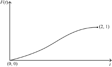
correct shape including correct concavity A1
clearly indicating starts at origin and ends at \((2,{\text{ }}1)\) A1
Note: Condone the absence of \((0,{\text{ }}0)\).
Note: Accept 2 on the \(x\)-axis and 1 on the \(y\)-axis correctly placed.
[2 marks]
attempt to solve \(\frac{{{a^2}}}{2} - \frac{{{a^4}}}{{16}} = 0.75\) (or equivalent) for \(a\) (M1)
\(a = 1.41{\text{ }}( = \sqrt 2 )\) A1
Note: Accept any answer that rounds to 1.4.
[2 marks]
Examiners report
The random variables \({X_1}\) and \({X_2}\) are a random sample from \({\text{N}}(\mu ,{\text{ 2}}{\sigma ^2})\). The random variables \({Y_1}\), \({Y_2}\) and \({Y_3}\) are a random sample from \({\text{N}}(2\mu ,{\text{ }}{\sigma ^2})\).
The estimator \(U\) is used to estimate \(\mu \) where \(U = a({X_1} + {X_2}) + b({Y_1} + {Y_2} + {Y_3})\) and \(a\), \(b\) are constants.
Given that \(U\) is unbiased, show that \(2a + 6b = 1\).
Show that \({\text{Var}}(U) = (39{b^2} - 12b + 1){\sigma ^2}\).
Hence find the value of \(a\) and the value of \(b\) which give the best unbiased estimator of this form, giving your answers as fractions.
Hence find the variance of this best unbiased estimator.
Markscheme
\({\text{E}}(U) = a\left( {{\text{E}}({X_1}) + {\text{E}}({X_2})} \right) + b\left( {{\text{E}}({Y_1}) + {\text{E}}({Y_2}) + {\text{E}}({Y_3})} \right)\) (M1)
\( = 2a\mu + 6b\mu \) A1
(for an unbiased estimator,) \({\text{E}}(U) = \mu \) R1
giving \(2a + 6b = 1\) AG
Note: Condone omission of E on LHS.
[3 marks]
\({\text{Var}}(U) = {a^2}\left( {{\text{Var}}({X_1}) + {\text{Var}}({X_2})} \right) + {b^2}\left( {{\text{Var}}({Y_1}) + {\text{Var}}({Y_2}) + {\text{Var}}({Y_3})} \right)\) (M1)
\( = 4{a^2}{\sigma ^2} + 3{b^2}{\sigma ^2}\) A1
\( = 4{\left( {\frac{{1 - 6b}}{2}} \right)^2}{\sigma ^2} + 3{b^2}{\sigma ^2}\) A1
\( = (39{b^2} - 12b + 1){\sigma ^2}\) AG
[3 marks]
the best unbiased estimator (of this form) will be found by minimising \({\text{Var}}(U)\) (R1)
For example, \(\frac{{\text{d}}}{{{\text{d}}b}}\left( {{\text{Var}}(U)} \right) = (78b - 12){\sigma ^2}\) (A1)
for a minimum, \(b = \frac{{12}}{{78}}\,\,\,\left( { = \frac{2}{{13}}} \right)\) so that \(a = \frac{3}{{78}}\,\,\,\left( { = \frac{1}{{26}}} \right)\) A1
[3 marks]
\({\text{Var}}U = \left( {39{{\left( {\frac{2}{{13}}} \right)}^2} - 12\left( {\frac{2}{{13}}} \right) + 1} \right){\sigma ^2}\)
\( = \frac{{{\sigma ^2}}}{{13}}\,\,\,(0.0769{\sigma ^2})\) A1
[1 mark]
Examiners report
The random variable X represents the height of a wave on a particular surf beach.
It is known that X is normally distributed with unknown mean \(\mu \) (metres) and known variance \({\sigma ^2} = \frac{1}{4}{\text{ (metre}}{{\text{s}}^2}{\text{)}}\) . Sally wishes to test the claim made in a surf guide that \(\mu = 3\) against the alternative that \(\mu < 3\) . She measures the heights of 36 waves and calculates their sample mean \({\bar x}\) . She uses this value to test the claim at the 5 % level.
(i) Find a simple inequality, of the form \(\bar x < A\) , where A is a number to be determined to 4 significant figures, so that Sally will reject the null hypothesis, that \(\mu = 3\) , if and only if this inequality is satisfied.
(ii) Define a Type I error.
(iii) Define a Type II error.
(iv) Write down the probability that Sally makes a Type I error.
(v) The true value of \(\mu \) is 2.75. Calculate the probability that Sally makes a Type II error.
The random variable Y represents the height of a wave on another surf beach. It is known that Y is normally distributed with unknown mean \(\mu \) (metres) and unknown variance \({\sigma ^2}{\text{ (metre}}{{\text{s}}^2}{\text{)}}\) . David wishes to test the claim made in a surf guide that \(\mu = 3\) against the alternative that \(\mu < 3\) . He is also going to perform this test at the 5 % level. He measures the heights of 36 waves and finds that the sample mean, \(\bar y = 2.860\) and the unbiased estimate of the population variance, \(s_{n - 1}^2 = 0.25\).
(i) State the name of the test that David should perform.
(ii) State the conclusion of David’s test, justifying your answer by giving the p-value.
(iii) Using David’s results, calculate the 90 % confidence interval for \(\mu \) , giving your answers to 4 significant figures.
Markscheme
(i) \({H_0}:\mu = 3,{\text{ }}{H_1}:\mu < 3\)
1 tailed z test as \({\sigma ^2}\) is known
under \({H_0}{\text{, }}X \sim {\text{N}}\left( {3,\frac{1}{4}} \right){\text{ so }}\bar X \sim {\text{N}}\left( {3,\frac{{\frac{1}{4}}}{{36}}} \right) = N\left( {3,\frac{1}{{144}}} \right)\) (M1)
\(z = \frac{{\bar x - 3}}{{\frac{1}{{12}}}}{\text{ is N(0, 1)}}\) (A1)
\({\text{P}}(z < - 1.64485...) = 0.05\) (A1)
so inequality is given by \(\frac{{\bar x - 3}}{{\frac{1}{{12}}}} < - 1.64485...{\text{ giving }}\bar x < 2.8629…\) M1
\(\bar x < 2.863{\text{ (4sf)}}\) A1
Note: Candidates can get directly to the answer from \({\text{N}}\left( {3,\frac{1}{{144}}} \right)\) they do not have to go via z is N(0, 1) . However they must give some explanation of what they have done; they cannot just write the answer down.
(ii) a Type I error is accepting \({H_1}\) when \({H_0}\) is true A1
(iii) a Type II error is accepting \({H_0}\) when \({H_1}\) is true A1
(iv) 0.05 A1
Note: Accept anything that rounds to 0.050 if they do the conditional calculation.
(v) \(\bar X \sim {\text{N}}\left( {2.75,\frac{1}{{144}}} \right)\) (M1)
\({\text{P}}(\bar x > 2.8629...) = 0.0877{\text{ (3sf)}}\) (M1)A1
Note: Accept any answer between 0.0875 and 0.0877 inclusive.
Note: Accept anything that rounded is between 0.087and 0.089 if there is evidence that the candidate has used tables.
[11 marks]
(i) t-test A1
(ii) \({{\text{H}}_0}:\mu = 3,{\text{ }}{{\text{H}}_1}:\mu < 3\)
1 tailed t test as \({\sigma ^2}\) is unknown
\(t = \frac{{\bar y - 3}}{{\frac{1}{{12}}}}\) has the t-distribution with \(v = 35\) (M1)
the p-value is 0.0509… A2
this is \( > 0.05\) R1
so we accept that the mean wave height is 3 R1
Note: Allow “Accept \({{\text{H}}_0}\) ” provided \({{\text{H}}_0}\) has been stated.
Note: Accept FT on the p-value for the R1s.
(iii) \(2.719 < \mu < 3.001{\text{ (4 sf)}}\) A1A1
Note: \(2.860 \pm 1.6896... \times \frac{{\frac{1}{2}}}{6}\) would gain M1.
Note: Award A1A0 if answer are only given to 3sf.
[8 marks]
Examiners report
(a) There were many reasonable answers. In (i) not all candidates explained their method so that they could gain good partial marks even if they had the wrong final answer. A common mistake was to give an answer above 3. It was pleasing that almost all candidates had (ii) and (iii) correct, as this had caused problems in the past. In (iv) it was amusing to see a few candidates work out 5% using conditional probability rather than just write down the answer as asked.
(b) It was pleasing that almost all candidates realised that it was a t-test rather than a z-test.
There was good understanding on how to use the calculator in parts (ii) and (iii). The correct confidence interval to the desired accuracy was not always given.
The most common mistake in question 3 was forgetting to take into account the variance of the sample mean.
A discrete random variable \(U\) follows a geometric distribution with \(p = \frac{1}{4}\).
Find \(F(u)\), the cumulative distribution function of \(U\), for \(u = 1,{\text{ }}2,{\text{ }}3 \ldots \)
Hence, or otherwise, find the value of \(P(U > 20)\).
Prove that the probability generating function of \(U\) is given by \({G_u}(t) = \frac{t}{{4 - 3t}}\).
Given that \({U_i} \sim {\text{Geo}}\left( {\frac{1}{4}} \right),{\text{ }}i = 1,{\text{ }}2,{\text{ }}3\), and that \(V = {U_1} + {U_2} + {U_3}\), find
(i) \({\text{E}}(V)\);
(ii) \({\text{Var}}(V)\);
(iii) \({G_v}(t)\), the probability generating function of \(V\).
A third random variable \(W\), has probability generating function \({G_w}(t) = \frac{1}{{{{(4 - 3t)}^3}}}\).
By differentiating \({G_w}(t)\), find \({\text{E}}(W)\).
A third random variable \(W\), has probability generating function \({G_w}(t) = \frac{1}{{{{(4 - 3t)}^3}}}\).
Prove that \(V = W + 3\).
Markscheme
METHOD 1
\({\text{P}}(U = u) = \frac{1}{4}{\left( {\frac{3}{4}} \right)^{u - 1}}\) (M1)
\(F(u) = {\text{P}}(U \le u) = \sum\limits_{r = 1}^u {\frac{1}{4}{{\left( {\frac{3}{4}} \right)}^{r - 1}}\;\;\;} \)(or equivalent)
\( = \frac{{\frac{1}{4}\left( {1 - {{\left( {\frac{3}{4}} \right)}^u}} \right)}}{{1 - \frac{3}{4}}}\) (M1)
\( = 1 - {\left( {\frac{3}{4}} \right)^u}\) A1
METHOD 2
\({\text{P}}(U \le u) = 1 - {\text{P}}(U > u)\) (M1)
\({\text{P}}(U > u) = \) probability of \(u\) consecutive failures (M1)
\({\text{P}}(U \le u) = 1 - {\left( {\frac{3}{4}} \right)^u}\) A1
[3 marks]
\({\text{P}}(U > 20) = 1 - {\text{P}}(U \le 20)\) (M1)
\( = {\left( {\frac{3}{4}} \right)^{20}}\;\;\;( = 0.00317)\) A1
[2 marks]
\({G_U}(t) = \sum\limits_{r = 1}^\infty {\frac{1}{4}{{\left( {\frac{3}{4}} \right)}^{r - 1}}{t^r}\;\;\;} \)(or equivalent) M1A1
\( = \sum\limits_{r = 1}^\infty {\frac{1}{3}{{\left( {\frac{3}{4}t} \right)}^r}} \) (M1)
\( = \frac{{\frac{1}{3}\left( {\frac{3}{4}t} \right)}}{{1 - \frac{3}{4}t}}\;\;\;\left( { = \frac{{\frac{1}{4}t}}{{1 - \frac{3}{4}t}}} \right)\) A1
\( = \frac{t}{{4 - 3t}}\) AG
[4 marks]
(i) \(E(U) = \frac{1}{{\frac{1}{4}}} = 4\) (A1)
\(E({U_1} + {U_2} + {U_3}{\text{)}} = 4 + 4 + 4 = 12\) A1
(ii) \({\text{Var}}(U) = \frac{{\frac{3}{4}}}{{{{\left( {\frac{1}{4}} \right)}^2}}}=12\) A1
\({\text{Var(}}{U_1} + {U_2} + {U_3}) = 12 + 12 + 12 = 36\) A1
(iii) \({G_v}(t) = {\left( {{G_U}(t)} \right)^3}\) (M1)
\( = {\left( {\frac{t}{{4 - 3t}}} \right)^3}\) A1
[6 marks]
\({G_W}^\prime (t) = - 3{(4 - 3t)^{ - 4}}( - 3)\;\;\;\left( { = \frac{9}{{{{(4 - 3t)}^4}}}} \right)\) (M1)(A1)
\(E(W) = {G_W}^\prime (1) = 9\) (M1)A1
Note: Allow the use of the calculator to perform the differentiation.
[4 marks]
EITHER
probability generating function of the constant 3 is \({t^3}\) A1
OR
\({G_{W - 3}}(t) = E({t^{W + 3}}) = E({t^W})E({t^3})\) A1
THEN
\(W + 3\) has generating function \({G_{W + 3}} = \frac{1}{{{{(4 - 3t)}^3}}} \times {t^3} = {G_V}(t)\) M1
as the generating functions are the same \(V = W + 3\) R1AG
[3 marks]
Total [22 marks]
Examiners report
The continuous random variable \(X\) has cumulative distribution function \(F\) given by \[F(x) = \left\{ {\begin{array}{*{20}{l}} {0,}&{x < 0} \\ {x{{\text{e}}^{x - 1}},}&{0 \leqslant x \leqslant 1.} \\ {1,}&{x > 2} \end{array}} \right.\]
Determine \(P(0.25 \leqslant X \leqslant 0.75)\);
Determine the median of \(X\).
Show that the probability density function \(f\) of \(X\) is given, for \(0 \leqslant x \leqslant 1\), by
\[f(x) = (x + 1){{\text{e}}^{x - 1}}.\]
Hence determine the mean and the variance of \(X\).
State the central limit theorem.
A random sample of 100 observations is obtained from the distribution of \(X\). If \(\bar X\) denotes the sample mean, use the central limit theorem to find an approximate value of \(P(\bar X > 0.65)\). Give your answer correct to two decimal places.
Markscheme
\(P(0.25 \leqslant X \leqslant 0.75) = F(0.75) - F(0.25)\) (M1)
\( = 0.466\) A1
Note: Accept any answer that rounds correctly to 0.466.
[2 marks]
the median \(m\) satisfies \(F(m) = 0.5\) (M1)
\(m = 0.685\) A1
Note: Accept any answer that rounds correctly to 0.685.
[2 marks]
\(f(x) = F’(x)\) (M1)
\( = {{\text{e}}^{x - 1}} + x{{\text{e}}^{x - 1}}\) A1
\( = (x + 1){{\text{e}}^{x - 1}}\) AG
[2 marks]
\(\mu = \int\limits_0^1 {x\left( {x + 1} \right){{\text{e}}^{x - 1}}{\text{d}}x} \) (M1)
\( = 0.632\,\,\,\left( {1 - \frac{1}{{\text{e}}}} \right)\) A1
Note: Accept any answer that rounds correctly to 0.632.
\({\sigma ^2} = \int\limits_0^1 {x\left( {x + 1} \right){{\text{e}}^{x - 1}}{\text{d}}x} - 0.632{ \ldots ^2}\) (M1)
\( = 0.0719\,\,\,\left( {\frac{6}{{\text{e}}} - 2 - \frac{1}{{{{\text{e}}^2}}}} \right)\) A1
Note: Accept any answer that rounds correctly to 0.072.
[4 marks]
the central limit theorem states that the mean of a large sample from any distribution (with a finite variance) is approximately normally distributed A1
[1 mark]
\(\bar X\) is approximately \(N(0.632 \ldots ,{\text{ }}0.000719 \ldots )\) (M1)(A1)
\(P(\bar X > 0.65) = 0.25\) (2 dps required) A1
[3 marks]
Examiners report
Adam does the crossword in the local newspaper every day. The time taken by Adam, \(X\) minutes, to complete the crossword is modelled by the normal distribution \({\text{N}}(22,{\text{ }}{5^2})\).
Beatrice also does the crossword in the local newspaper every day. The time taken by Beatrice, \(Y\) minutes, to complete the crossword is modelled by the normal distribution \({\text{N}}(40,{\text{ }}{6^2})\).
Given that, on a randomly chosen day, the probability that he completes the crossword in less than \(a\) minutes is equal to 0.8, find the value of \(a\).
Find the probability that the total time taken for him to complete five randomly chosen crosswords exceeds 120 minutes.
Find the probability that, on a randomly chosen day, the time taken by Beatrice to complete the crossword is more than twice the time taken by Adam to complete the crossword. Assume that these two times are independent.
Markscheme
\(z = 0.841 \ldots \) (A1)
\(a = \mu + z\sigma \) (M1)
\( = 26.2\) A1
[3 marks]
let \(T\) denote the total time taken to complete 5 crosswords.
\(T\) is \({\text{N}}(110,{\text{ }}125)\) (A1)(A1)
Note: A1 for the mean and A1 for the variance.
\({\text{P}}(T > 120) = 0.186\) A1
[3 marks]
consider the random variable \(U = Y - 2X\) (M1)
\({\text{E}}(U) = - 4\) A1
\({\text{Var}}(U) = {\text{Var}}(Y) + 4{\text{Var}}(X)\) (M1)
\( = 136\) A1
\({\text{P}}(Y > 2X) = {\text{P}}(U > 0)\) (M1)
\( = 0.366\) A1
[6 marks]
Examiners report
Part (a) was very well answered with only a very few weak candidates using 0.8 instead of 0.841...
Part (b) was well answered with only a few candidates calculating the variance incorrectly.
Part (c) was again well answered. The most common errors, not often seen, were writing the variance of \(Y - 2X\) as either \({\text{Var}}(Y) + 2{\text{Var}}(X)\) or \({\text{Var}}(Y) - 2(or{\text{ }}4){\text{Var}}(X)\).
The random variables \(X\), \(Y\) follow a bivariate normal distribution with product moment correlation coefficient \(\rho \).
A random sample of 10 observations on \(X\), \(Y\) was obtained and the value of \(r\), the sample product moment correlation coefficient, was calculated to be 0.486.
State suitable hypotheses to investigate whether or not \(X\), \(Y\) are independent.
(i) Determine the \(p\)-value.
(ii) State your conclusion at the 5% significance level.
Explain why the equation of the regression line of \(y\) on \(x\) should not be used to predict the value of \(y\) corresponding to \(x = {x_0}\), where \({x_0}\) lies within the range of values of \(x\) in the sample.
Markscheme
\({H_0}:{\text{ }}\rho = 0;{\text{ }}{H_1}:{\text{ }}\rho \ne 0\) A1A1
[2 marks]
(i) \(t = 0.486 \times \sqrt {\frac{{10 - 2}}{{1 - {{0.486}^2}}}} \) (M1)
\( = 1.572 \ldots \) (A1)
degrees of freedom \( = 8\) (A1)
\({\text{P}}(T > 1.5728 \ldots )\) (M1)
\( = 0.0772\) (A1)
\(p{\text{ - value }} = {\text{ }}0.154\) A1
Note: Do not follow through for the final A1 if their \({H_1}\) is one-sided.
(ii) accept \({H_0}\) or equivalent statement involving \({H_0}\) or \({H_1}\) (at the 5% significance level) R1
Note: Follow through the candidate’s \(p\)-value.
[7 marks]
EITHER
because the above analysis suggests that \(X\), \(Y\) are independent R1
OR
the value of \(r\) suggests that \(X\) and \(Y\) are weakly correlated R1
[1 mark]
Examiners report
Part (a) was well answered with only a few candidates using inappropriate symbols, for example \(r\) or \(\mu \). Also, only very few candidates failed to realise that the wording of the question indicated that a two-tailed test was required.
The test in (b) was generally well carried out and the \(p\)-value found correctly. The most common errors were using incorrect degrees of freedom and evaluating a one-tailed \(p\)-value instead of a two-tailed \(p\)-value.
In (c), many realised that the earlier work meant that the regression line should not be used because the variables had been found to be independent. Incorrect reasons, however, were not uncommon, for example the suggestions that either the regression line of \(x\) on \(y\) should be used or that there were insufficient data.
John rings a church bell 120 times. The time interval, \({T_i}\), between two successive rings is a random variable with mean of 2 seconds and variance of \(\frac{1}{9}{\text{ second}}{{\text{s}}^2}\).
Each time interval, \({T_i}\), is independent of the other time intervals. Let \(X = \sum\limits_{i = 1}^{119} {{T_i}} \) be the total time between the first ring and the last ring.
The church vicar subsequently becomes suspicious that John has stopped coming to ring the bell and that he is letting his friend Ray do it. When Ray rings the bell the time interval, \({T_i}\) has a mean of 2 seconds and variance of \(\frac{1}{{25}}{\text{ second}}{{\text{s}}^2}\).
The church vicar makes the following hypotheses:
\({H_0}\): Ray is ringing the bell; \({H_1}\): John is ringing the bell.
He records four values of \(X\). He decides on the following decision rule:
If \(236 \leqslant X \leqslant 240\) for all four values of \(X\) he accepts \({H_0}\), otherwise he accepts \({H_1}\).
Find
(i) \({\text{E}}(X)\);
(ii) \({\text{Var}}(X)\).
Explain why a normal distribution can be used to give an approximate model for \(X\).
Use this model to find the values of \(A\) and \(B\) such that \({\text{P}}(A < X < B) = 0.9\), where \(A\) and \(B\) are symmetrical about the mean of \(X\).
Calculate the probability that he makes a Type II error.
Markscheme
(i) \({\text{mean}} = 119 \times 2 = 238\) A1
(ii) \({\text{variance}} = 119 \times \frac{1}{9} = \frac{{119}}{9}{\text{ }}( = 13.2)\) (M1)A1
Note: If 120 is used instead of 119 award A0(M1)A0 for part (a) and apply follow through for parts (b)-(d). (b) is unaffected and in (c) the interval becomes \((234,{\text{ }}246)\). In (d) the first 2 A1 marks are for \(0.3633 \ldots \) and \(0.0174 \ldots \) so the final answer will round to 0.017.
[3 marks]
justified by the Central Limit Theorem R1
since \(n\) is large A1
Note: Accept \(n > 30\).
[2 marks]
\(X \sim N\left( {238,{\text{ }}\frac{{119}}{9}} \right)\)
\(Z = \frac{{X - 238}}{{\frac{{\sqrt {119} }}{3}}} \sim N(0,{\text{ }}1)\) (M1)(A1)
\({\text{P}}(Z < q) = 0.95 \Rightarrow q = 1.644 \ldots \) (A1)
so \({\text{P}}( - 1.644 \ldots < Z < 1.644 \ldots ) = 0.9\) (R1)
\({\text{P}}( - 1.644 \ldots < \frac{{X - 238}}{{\frac{{\sqrt {119} }}{3}}} < 1.644 \ldots ) = 0.9\) (M1)
interval is \(232 < X < 244{\text{ }}({\text{3sf}}){\text{ }}(A = 232,{\text{ }}B = 244)\) A1A1
Notes: Accept the use of inverse normal applied to the distribution of \(X\).
Alternative is to use the GDC to find a pretend \(Z\) confidence interval for a mean and then convert by multiplying by 119.
Either \(A\) or \(B\) correct implies the five implied marks.
Accept any numbers that round to these 3sf numbers.
[7 marks]
under \({{\text{H}}_1},{\text{ }}X \sim N\left( {238,{\text{ }}\frac{{119}}{9}} \right)\) (M1)
\({\text{P}}(236 \leqslant X \leqslant 240) = 0.41769 \ldots \) (A1)
probability that all 4 values of \(X\) lie in this interval is
\({(0.41769 \ldots )^4} = 0.030439 \ldots \) (M1)(A1)
so probability of a Type II error is 0.0304 (3sf) A1
Note: Accept any answer that rounds to 0.030.
[5 marks]
Examiners report
The random variables X , Y follow a bivariate normal distribution with product moment correlation coefficient ρ.
A random sample of 11 observations on X, Y was obtained and the value of the sample product moment correlation coefficient, r, was calculated to be −0.708.
The covariance of the random variables U, V is defined by
Cov(U, V) = E((U − E(U))(V − E(V))).
State suitable hypotheses to investigate whether or not a negative linear association exists between X and Y.
Determine the p-value.
State your conclusion at the 1 % significance level.
Show that Cov(U, V) = E(UV) − E(U)E(V).
Hence show that if U, V are independent random variables then the population product moment correlation coefficient, ρ, is zero.
Markscheme
H0 : ρ = 0; H1 : ρ < 0 A1
[1 mark]
\(t = - 0.708\sqrt {\frac{{11 - 2}}{{1 - {{\left( { - 0.708} \right)}^2}}}} \,\, = \,\,\left( { - 3.0075 \ldots } \right)\) (M1)
degrees of freedom = 9 (A1)
P(T < −3.0075...) = 0.00739 A1
Note: Accept any answer that rounds to 0.0074.
[3 marks]
reject H0 or equivalent statement R1
Note: Apply follow through on the candidate’s p-value.
[1 mark]
Cov(U, V) + E((U − E(U))(V − E(V)))
= E(UV − E(U)V − E(V)U + E(U)E(V)) M1
= E(UV) − E(E(U)V) − E(E(V)U) + E(E(U)E(V)) (A1)
= E(UV) − E(U)E(V) − E(V)E(U) + E(U)E(V) A1
Cov(U, V) = E(UV) − E(U)E(V) AG
[3 marks]
E(UV) = E(U)E(V) (independent random variables) R1
⇒Cov(U, V) = E(U)E(V) − E(U)E(V) = 0 A1
hence, ρ = \(\frac{{{\text{Cov}}\left( {U,\,V} \right)}}{{\sqrt {{\text{Var}}\left( U \right)\,{\text{Var}}\left( V \right)} }} = 0\) A1AG
Note: Accept the statement that Cov(U,V) is the numerator of the formula for ρ.
Note: Only award the first A1 if the R1 is awarded.
[3 marks]
Examiners report
A smartphone’s battery life is defined as the number of hours a fully charged battery can be used before the smartphone stops working. A company claims that the battery life of a model of smartphone is, on average, 9.5 hours. To test this claim, an experiment is conducted on a random sample of 20 smartphones of this model. For each smartphone, the battery life, \(b\) hours, is measured and the sample mean, \({\bar b}\), calculated. It can be assumed the battery lives are normally distributed with standard deviation 0.4 hours.
It is then found that this model of smartphone has an average battery life of 9.8 hours.
State suitable hypotheses for a two-tailed test.
Find the critical region for testing \({\bar b}\) at the 5 % significance level.
Find the probability of making a Type II error.
Another model of smartphone whose battery life may be assumed to be normally distributed with mean μ hours and standard deviation 1.2 hours is tested. A researcher measures the battery life of six of these smartphones and calculates a confidence interval of [10.2, 11.4] for μ.
Calculate the confidence level of this interval.
Markscheme
Note: In question 3, accept answers that round correctly to 2 significant figures.
\({{\text{H}}_0}\,{\text{:}}\,\mu = 9.5{\text{;}}\,\,{{\text{H}}_1}\,{\text{:}}\,\mu \ne 9.5\) A1
[1 mark]
Note: In question 3, accept answers that round correctly to 2 significant figures.
the critical values are \(9.5 \pm 1.95996 \ldots \times \frac{{0.4}}{{\sqrt {20} }}\) (M1)(A1)
i.e. 9.3247…, 9.6753…
the critical region is \({\bar b}\) < 9.32, \({\bar b}\) > 9.68 A1A1
Note: Award A1 for correct inequalities, A1 for correct values.
Note: Award M0 if t-distribution used, note that t(19)97.5 = 2.093 …
[4 marks]
Note: In question 3, accept answers that round correctly to 2 significant figures.
\(\bar B \sim {\text{N}}\left( {9.8,\,{{\left( {\frac{{0.4}}{{\sqrt {20} }}} \right)}^2}} \right)\) (A1)
\({\text{P}}\left( {9.3247 \ldots < \bar B < 9.6753 \ldots } \right)\) (M1)
=0.0816 A1
Note: FT the critical values from (b). Note that critical values of 9.32 and 9.68 give 0.0899.
[3 marks]
Note: In question 3, accept answers that round correctly to 2 significant figures.
METHOD 1
\(X \sim {\text{N}}\left( {{\text{10}}{\text{.8,}}\,\frac{{{{1.2}^2}}}{6}} \right)\) (M1)(A1)
P(10.2 < X < 11.4) = 0.7793… (A1)
confidence level is 77.9% A1
Note: Accept 78%.
METHOD 2
\(11.4 - 10.2 = 2z \times \frac{{1.2}}{{\sqrt 6 }}\) (M1)
\(z = 1.224 \ldots \) (A1)
P(−1.224… < Z < 1.224…) = 0.7793… (A1)
confidence level is 77.9% A1
Note: Accept 78%.
[4 marks]
Examiners report
The random variable X has the negative binomial distribution NB(5, p), where p < 0.5, and \({\text{P}}(X = 10) = 0.05\). By first finding the value of p, find the value of \({\text{P}}(X = 11)\).
Markscheme
\({\text{P}}(X = 10) = \left( {\begin{array}{*{20}{c}}
9 \\
4
\end{array}} \right){p^5}{(1 - p)^5}\) (= 0.05) (M1)A1A1
Note: First A1 is for the binomial coefficient. Second A1 is for the rest.
solving by any method, \(p = 0.297 \ldots \) A4
Notes: Award A2 for anything which rounds to 0.703.
Do not apply any AP at this stage.
\({\text{P}}(X = 10) = \left( {\begin{array}{*{20}{c}}
{10} \\
4
\end{array}} \right) \times {(0.297...)^5} \times {(1 - 0.297...)^6}\) (M1)A1
= 0.0586 A1
Note: Allow follow through for incorrect p-values.
[10 marks]
Examiners report
Questions on these discrete distributions have not been generally well answered in the past and it was pleasing to note that many candidates submitted a reasonably good solution to this question. In (b), the determination of the value of p was often successful using a variety of methods including solving the equation \(p(1 - p) = {(0.000396{\text{ }} \ldots )^{1/5}}\), graph plotting or using SOLVER on the GDC or even expanding the equation into a \({10^{{\text{th}}}}\) degree polynomial and solving that. Solutions to this particular question exceeded expectations.
The weights of adult monkeys of a certain species are known to be normally distributed, the males with mean 30 kg and standard deviation 3 kg and the females with mean 20 kg and standard deviation 2.5 kg.
Find the probability that the weight of a randomly selected male is more than twice the weight of a randomly selected female.
Two males and five females stand together on a weighing machine. Find the probability that their total weight is less than 175 kg.
Markscheme
we are given that \(M \sim {\text{N(30, 9)}}\) and \(F \sim {\text{N(20, 6.25)}}\)
let \(X = M - 2F;{\text{ }}X \sim {\text{N}}\)(\( - 10\), \(34\)) M1A1A1
we require \({\text{P}}(X > 0)\) (M1)
= 0.0432 A1
[5 marks]
let \(Y = {M_1} + {M_2} + {F_1} + {F_2} + {F_3} + {F_4} + {F_5};{\text{ }}Y \sim {\text{N(160, 49.25)}}\) M1A1A1
we require \({\text{P}}(Y < 175) = 0.984\) A1
[4 marks]
Examiners report
A teacher decides to use the marks obtained by a random sample of 12 students in Geography and History examinations to investigate whether or not there is a positive association between marks obtained by students in these two subjects. You may assume that the distribution of marks in the two subjects is bivariate normal.
He gives the marks to Anne, one of his students, and asks her to use a calculator to carry out an appropriate test at the 5% significance level. Anne reports that the \(p\)-value is 0.177.
State suitable hypotheses for this investigation.
State, in context, what conclusion should be drawn from this \(p\)-value.
The teacher then asks Anne for the values of the \(t\)-statistic and the product moment correlation coefficient \(r\) produced by the calculator but she has deleted these. Starting with the \(p\)-value, calculate these values of \(t\) and \(r\).
Markscheme
\({H_0}:\rho = 0;{\text{ }}{H_1}:\rho > 0\) A1
Note: Do not accept \(r\) in place of \(\rho \).
[1 mark]
insufficient evidence to conclude that there is a (positive) association between marks in these two subjects (or equivalent statement in context) A1
[1 mark]
degrees of freedom \( = 10\) (A1)
required value of \(t = {\text{inverse }}t(0.823)\) (M1)
\( = 0.972\) A1
attempt to solve \(t = r\sqrt {\frac{{n - 2}}{{1 - {r^2}}}} \) (M1)
\(r = 0.294\) A1
Note: Accept any \(r\) value that rounds to 0.29.
Note: Follow through their \(t\) value to determine \(r\).
[5 marks]
Examiners report
(a) The heating in a residential school is to be increased on the third frosty day during the term. If the probability that a day will be frosty is 0.09, what is the probability that the heating is increased on the \({25^{{\text{th}}}}\) day of the term?
(b) On which day is the heating most likely to be increased?
Markscheme
(a) the distribution is NB(3, 0.09) (M1)(A1)
the probability is \(\left( {\begin{array}{*{20}{c}}
{24} \\
2
\end{array}} \right){0.91^{22}} \times {0.09^3} = 0.0253\) (M1)(A1)A1
[5 marks]
(b) P(Heating increased on \({n^{{\text{th}}}}\) day)
\(\left( {\begin{array}{*{20}{c}}
{n - 1} \\
2
\end{array}} \right){0.91^{n - 3}} \times {0.09^3}\) (M1)(A1)(A1)
by trial and error n = 23 gives the maximum probability (M1)A3
(neighbouring values: 0.02551 (n = 22) ; 0.02554 (n = 23) ; 0.02545 (n = 24) )
[7 marks]
Total [12 marks]
Examiners report
Most candidates understood the context of this question, and the negative binomial distribution was usually applied, albeit occasionally with incorrect parameters. Good solutions were seen to part(b), using lists in their GDC or trial and error.
If \(X\) and \(Y\) are two random variables such that \({\text{E}}(X) = {\mu _X}\) and \({\text{E}}(Y) = {\mu _Y}\) then \({\text{Cov}}(X,{\text{ }}Y) = {\text{E}}\left( {(X - {\mu _X})(Y - {\mu _Y})} \right)\).
Prove that if \(X\) and \(Y\) are independent then \({\text{Cov}}(X,{\text{ }}Y) = 0\).
In a particular company, it is claimed that the distance travelled by employees to work is independent of their salary. To test this, 20 randomly selected employees are asked about the distance they travel to work and the size of their salaries. It is found that the product moment correlation coefficient, \(r\), for the sample is \( - 0.35\).
You may assume that both salary and distance travelled to work follow normal distributions.
Perform a one-tailed test at the \(5\% \) significance level to test whether or not the distance travelled to work and the salaries of the employees are independent.
Markscheme
METHOD 1
\({\text{Cov}}(X,{\text{ }}Y) = {\text{E}}\left( {(X - {\mu _X})(Y - {\mu _Y})} \right)\)
\( = {\text{E}}(XY - X{\mu _Y} - Y{\mu _X} + {\mu _X}{\mu _Y})\) (M1)
\( = {\text{E}}(XY) - {\mu _Y}{\text{E}}(X) - {\mu _X}{\text{E}}(Y) + {\mu _X}{\mu _Y}\)
\( = {\text{E}}(XY) - {\mu _X}{\mu _Y}\) A1
as \(X\) and \(Y\) are independent \({\text{E}}(XY) = {\mu _X}{\mu _Y}\) R1
\({\text{Cov}}(X,{\text{ }}Y) = 0\) AG
METHOD 2
\({\text{Cov}}(X,{\text{ }}Y) = {\text{E}}\left( {(X - {\mu _x})(Y - {\mu _y})} \right)\)
\( = {\text{E}}(X - {\mu _x}){\text{E}}(Y - {\mu _y})\) (M1)
since \(X,Y\) are independent R1
\( = ({\mu _x} - {\mu _x})({\mu _y} - {\mu _y})\) A1
\( = 0\) AG
[3 marks]
\({H_0}:\rho = 0\;\;\;{H_1}:\rho < 0\) A1
Note: The hypotheses must be expressed in terms of \(\rho \).
test statistic \({t_{test}} = - 0.35\sqrt {\frac{{20 - 2}}{{1 - {{( - 0.35)}^2}}}} \) (M1)(A1)
\( = - 1.585 \ldots \) (A1)
\({\text{degrees of freedom}} = 18\) (A1)
EITHER
\(p{\text{ - value}} = 0.0652\) A1
this is greater than \(0.05\) M1
OR
\({t_{5\% }}(18) = - 1.73\) A1
this is less than \( - {\text{1.59}}\) M1
THEN
hence accept \({H_0}\) or reject \({H_1}\) or equivalent or contextual equivalent R1
Note: Allow follow through for the final R1 mark.
[8 marks]
Total [11 marks]
Examiners report
Solutions to (a) were often disappointing with few candidates gaining full marks, a common error being failure to state that
\(E(XY) = E(X)E(Y)\) or \({\text{E}}\left( {(X - {\mu _x})(Y - {\mu _y})} \right) = {\text{E}}(X - {\mu _x}){\text{E}}(Y - {\mu _y})\) in the case of independence.
In (b), the hypotheses were sometimes given incorrectly. Some candidates gave \({H_1}\) as \(\rho \ne 0\), not seeing that a one-tailed test was required. A more serious error was giving the hypotheses as \({H_0}:r = 0,{\text{ }}{H_1}:r < 0\) which shows a complete misunderstanding of the situation. Subsequent parts of the question were well answered in general.
Consider the recurrence relation
\({u_n} = 5{u_{n - 1}} - 6{u_{n - 2}},{\text{ }}{u_0} = 0\) and \({u_1} = 1\).
Find an expression for \({u_n}\) in terms of \(n\).
For every prime number \(p > 3\), show that \(p|{u_{p - 1}}\).
Markscheme
the auxiliary equation is \({\lambda ^2} - 5\lambda + 6 = 0\) M1
\( \Rightarrow \lambda = 2,{\text{ }}3\) (A1)
the general solution is \({u_n} = A \times {2^n} + B \times {3^n}\) A1
imposing initial conditions (substituting \(n = 0,{\text{ }}1\)) M1
\(A + B = 0\) and \(2A + 3B = 1\) A1
the solution is \(A = - 1,{\text{ }}B = 1\)
so that \({u_n} = {3^n} - {2^n}\) A1
[6 marks]
\({u_{p - 1}} = {3^{p - 1}} - {2^{p - 1}}\)
\(p > 3\), therefore 3 or 2 are not divisible by \(p\) R1
hence by FLT, \({3^{p - 1}} \equiv 1 \equiv {2^{p - 1}}(\bmod p)\) for \(p > 3\) M1A1
\({u_{p - 1}} \equiv 0(\bmod p)\) A1
\(p|{u_{p - 1}}\) for every prime number \(p > 3\) AG
[4 marks]
Examiners report
The students in a class take an examination in Applied Mathematics which consists of two papers. Paper 1 is in Mechanics and Paper 2 is in Statistics. The marks obtained by the students in Paper 1 and Paper 2 are denoted by \((x,{\text{ }}y)\) respectively and you may assume that the values of \((x,{\text{ }}y)\) form a random sample from a bivariate normal distribution with correlation coefficient \(\rho \) . The teacher wishes to determine whether or not there is a positive association between marks in Mechanics and marks in Statistics.
State suitable hypotheses.
The marks obtained by the 12 students who sat both papers are given in the following table.

(i) Determine the product moment correlation coefficient for these data and state its p-value.
(ii) Interpret your p-value in the context of the problem.
George obtained a mark of 63 on Paper 1 but was unable to sit Paper 2 because of illness. Predict the mark that he would have obtained on Paper 2.
Another class of 16 students sat examinations in Physics and Chemistry and the product moment correlation coefficient between the marks in these two subjects was calculated to be 0.524. Using a 1 % significance level, determine whether or not this value suggests a positive association between marks in Physics and marks in Chemistry.
Markscheme
\({{\text{H}}_0}:\rho = 0;{\text{ }}{{\text{H}}_1}:\rho > 0\) A1
[1 mark]
(i) correlation coefficient = 0.905 A2
p-value \( = 2.61 \times {10^{ - 5}}\) A2
(ii) very strong evidence to indicate a positive association between marks in Mechanics and marks in Statistics R1
[5 marks]
the regression line of y on x is \(y = 8.71 + 0.789x\) (M1)A1
George’s estimated mark on Paper 2 \( = 8.71 + 0.789 \times 63\) (M1)
= 58 A1
[4 marks]
\(t = r\sqrt {\frac{{n - 2}}{{1 - {r^2}}}} = 2.3019 \ldots \) M1A1
degrees of freedom = 14 (A1)
p-value \( = 0.0186 \ldots \) A1
at the 1 % significance level, this does not indicate a positive association between the marks in Physics and Chemistry R1
[5 marks]
Examiners report
The random variable X has a Poisson distribution with unknown mean \(\mu \) . It is required to test the hypotheses
\({H_0}:\mu = 3\) against \({H_1}:\mu \ne 3\) .
Let S denote the sum of 10 randomly chosen values of X . The critical region is defined as \((S \leqslant 22) \cup (S \geqslant 38)\) .
Calculate the significance level of the test.
Given that the value of \(\mu \) is actually 2.5, determine the probability of a Type II error.
Markscheme
under \({H_0}\) , \(S{\text{ is Po}}(30)\) (A1)
EITHER
\({\text{P}}(S \leqslant 22) = {\text{0.080569}} \ldots \) A1
\({\text{P}}(S \geqslant 38) = {\text{0.089012}} \ldots \) A1
significance level = 0.080569… + 0.089012… (M1)
= 0.170 A1
OR
\({\text{P}}(S \leqslant 22) = {\text{0.080569}} \ldots \) A1
\({\text{P}}(S \leqslant 37) = {\text{0.910987}} \ldots \) A1
significance level = 1 – (0.910987…) + 0.089012… (M1)
= 0.170 A1
Note: Accept 17 % or 0.17.
Note: Award 2 marks out of the final 4 marks for correct use of the Central Limit Theorem, giving 0.144 without a continuity correction and 0.171 with a continuity correction. The first (A1) is independent.
[5 marks]
S is now Po(25) (A1)
P (Type II error) = P (accept \({H_0}|\mu = 2.5\)) (M1)
\( = {\text{P}}\left( {23 \leqslant S \leqslant 37|S{\text{ is Po}}(25)} \right)\) (M1)
Note: Only one of the above M1 marks can be implied.
= 0.990789… – 0.317533… (A1)
= 0.673 A1
Note: Award 2 marks out of the final 4 marks for correct use of the Central Limit Theorem, giving 0.647 without a continuity correction and 0.685 with a continuity correction. The first (A1) is independent.
[5 marks]
Examiners report
Solutions to this question were often disappointing with many candidates not knowing what had to be done. Even those candidates who knew what to do sometimes made errors in evaluating the probabilities, often by misinterpreting the inequality signs. Candidates who used the Central Limit Theorem to evaluate the probabilities were given only partial credit on the grounds that the answers obtained were approximate and not exact.
Solutions to this question were often disappointing with many candidates not knowing what had to be done. Even those candidates who knew what to do sometimes made errors in evaluating the probabilities, often by misinterpreting the inequality signs. Candidates who used the Central Limit Theorem to evaluate the probabilities were given only partial credit on the grounds that the answers obtained were approximate and not exact.
The following table gives the average yield of olives per tree, in kg, and the rainfall, in cm, for nine separate regions of Greece. You may assume that these data are a random sample from a bivariate normal distribution, with correlation coefficient \(\rho \).
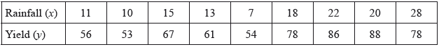
A scientist wishes to use these data to determine whether there is a positive correlation between rainfall and yield.
(a) State suitable hypotheses.
(b) Determine the product moment correlation coefficient for these data.
(c) Determine the associated p-value and comment on this value in the context of the question.
(d) Find the equation of the regression line of y on x.
(e) Hence, estimate the yield per tree in a tenth region where the rainfall was 19 cm.
(f) Determine the angle between the regression line of y on x and that of x on y . Give your answer to the nearest degree.
Markscheme
(a) \({H_0}:\rho = 0\) A1
\({H_1}:\rho > 0\) A1
[2 marks]
(b) 0.853 A2
Note: Accept any answer that rounds to 0.85.
[2 marks]
(c) p-value = 0.00173 (1-tailed) A1
Note: Accept any answer that rounds to 0.0017.
Accept any answer that rounds to 0.0035 obtained from 2-tailed test.
strong evidence to reject the hypothesis that there is no correlation between rainfall and yield or to accept the hypothesis that there is correlation between rainfall and yield R1
Note: Follow through the p-value for the conclusion.
[2 marks]
(d) \(y = 1.78x + 40.5\) A1A1
Note: Accept numerical coefficients that round to 1.8 and 41.
[2 marks]
(e) \(y = 1.77 \ldots (19) + 14.5 \ldots \) M1
74.3 A1
Note: Accept any answer that rounds to 74 or 75.
[2 marks]
(f) the gradient of the regression line y on x is 1.78 or equivalent A1
the regression line of x on y is \(x = 0.409y - 12.2\) (A1)
the gradient of the regression line x on y is \(\frac{1}{{0.409}}{\text{ }}( = 2.44)\) (M1)A1
calculate \(\arctan (2.44) - \arctan (1.78)\) (M1)
angle between regression lines is 7 degrees A1
Note: Accept any answer which rounds to ±7 degrees.
[6 marks]
Total [16 marks]
Examiners report
A farmer sells bags of potatoes which he states have a mean weight of 7 kg . An inspector, however, claims that the mean weight is less than 7 kg . In order to test this claim, the inspector takes a random sample of 12 of these bags and determines the weight, \(x\) kg , of each bag. He finds that \[\sum {x = 83.64;{\text{ }}\sum {{x^2} = 583.05.} } \] You may assume that the weights of the bags of potatoes can be modelled by the normal distribution \({\text{N}}(\mu ,{\text{ }}{\sigma ^2})\).
State suitable hypotheses to test the inspector’s claim.
Find unbiased estimates of \(\mu \) and \({\sigma ^2}\).
Carry out an appropriate test and state the \(p\)-value obtained.
Using a 10% significance level and justifying your answer, state your conclusion in context.
Markscheme
\({H_0}:\mu = 7,{\text{ }}{H_1}:\mu < 7\) A1
[1 mark]
\(\bar x = \frac{{83.64}}{{12}} = 6.97\) A1
\(s_{n - 1}^2 = \frac{{583.05}}{{11}} - \frac{{{\text{ }}{{83.64}^2}}}{{132}} = 0.0072\) (M1)A1
[3 marks]
\(t = \frac{{6.97 - 7}}{{\sqrt {\frac{{0.0072}}{{12}}} }} = - 1.22(474 \ldots )\) (M1)(A1)
\({\text{degrees of freedom}} = 11\) (A1)
\(p{\text{ - value}} = 0.123\) A1
Note: Accept any answer that rounds correctly to 0.12.
[4 marks]
because \(p > 0.1\) R1
the inspector’s claim is not supported (at the 10% level)
(or equivalent in context) A1
Note: Only award the A1 if the R1 has been awarded
[2 marks]
Examiners report
The random variable X represents the lifetime in hours of a battery. The lifetime may be assumed to be a continuous random variable X with a probability density function given by \(f(x) = \lambda {{\text{e}}^{ - \lambda x}}\), where \(x \geqslant 0\).
Find the cumulative distribution function, \(F(x)\), of X.
Find the probability that the lifetime of a particular battery is more than twice the mean.
Find the median of X in terms of \(\lambda \).
Find the probability that the lifetime of a particular battery lies between the median and the mean.
Markscheme
\(\int {\lambda {{\text{e}}^{ - \lambda t}}{\text{d}}t = - {{\text{e}}^{ - \lambda t}}{\text{ }}( + c)} \) A1
\( \Rightarrow F(x) = \left[ { - {{\text{e}}^{ - \lambda t}}} \right]_0^x\) (M1)
\( = 1 - {{\text{e}}^{ - \lambda t}}{\text{ }}(x \geqslant 0)\) A1
[3 marks]
\(1 - F\left( {\frac{2}{\lambda }} \right)\) M1
\( = {{\text{e}}^{ - 2}}\,\,\,\,\,( = 0.135)\) A1
[2 marks]
\(F(m) = \frac{1}{2}\) (M1)
\( \Rightarrow {{\text{e}}^{ - \lambda m}} = \frac{1}{2}\) A1
\( \Rightarrow - \lambda m = \ln \frac{1}{2}\)
\( \Rightarrow m = \frac{1}{\lambda }\ln 2\) A1
[3 marks]
\(F\left( {\frac{1}{\lambda }} \right) - F\left( {\frac{{\ln 2}}{\lambda }} \right)\) M1
\( = \frac{1}{2} - {{\text{e}}^{ - 1}}\,\,\,\,\,( = 0.132)\) A1
[2 marks]
Examiners report
For most candidates the question started well, but many did not appear to understand how to find the cumulative distribution function in (b). Many were able to integrate \(\lambda {{\text{e}}^{ - \lambda x}}\), but then did not know what to do with the integral. Parts (c), (d) and (e) were relatively well done, but even candidates who successfully found the cumulative distribution function often did not use it. This resulted in a lot of time spent integrating the same function.
For most candidates the question started well, but many did not appear to understand how to find the cumulative distribution function in (b). Many were able to integrate \(\lambda {{\text{e}}^{ - \lambda x}}\), but then did not know what to do with the integral. Parts (c), (d) and (e) were relatively well done, but even candidates who successfully found the cumulative distribution function often did not use it. This resulted in a lot of time spent integrating the same function.
For most candidates the question started well, but many did not appear to understand how to find the cumulative distribution function in (b). Many were able to integrate \(\lambda {{\text{e}}^{ - \lambda x}}\), but then did not know what to do with the integral. Parts (c), (d) and (e) were relatively well done, but even candidates who successfully found the cumulative distribution function often did not use it. This resulted in a lot of time spent integrating the same function.
For most candidates the question started well, but many did not appear to understand how to find the cumulative distribution function in (b). Many were able to integrate \(\lambda {{\text{e}}^{ - \lambda x}}\), but then did not know what to do with the integral. Parts (c), (d) and (e) were relatively well done, but even candidates who successfully found the cumulative distribution function often did not use it. This resulted in a lot of time spent integrating the same function.
Anne is a farmer who grows and sells pumpkins. Interested in the weights of pumpkins produced, she records the weights of eight pumpkins and obtains the following results in kilograms.
\[{\text{7.7}}\quad {\text{7.5}}\quad {\text{8.4}}\quad {\text{8.8}}\quad {\text{7.3}}\quad {\text{9.0}}\quad {\text{7.8}}\quad {\text{7.6}}\]
Assume that these weights form a random sample from a \(N(\mu ,{\text{ }}{\sigma ^2})\) distribution.
Anne claims that the mean pumpkin weight is 7.5 kilograms. In order to test this claim, she sets up the null hypothesis \({{\text{H}}_0}:\mu = 7.5\).
Determine unbiased estimates for \(\mu \) and \({\sigma ^2}\).
Use a two-tailed test to determine the \(p\)-value for the above results.
Interpret your \(p\)-value at the 5% level of significance, justifying your conclusion.
Markscheme
UE of \(\mu \) is \(8.01{\text{ }}( = 8.0125)\) A1
UE of \({\sigma ^2}\) is 0.404 (M1)A1
Note: Accept answers that round correctly to 2 sf.
Note: Condone incorrect notation, ie, \(\mu \) instead of UE of \(\mu \) and \({\sigma ^2}\) instead of UE of \({\sigma ^2}\).
Note: M0 for squaring \(0.594 \ldots \) giving 0.354, M1A0 for failing to square \(0.635 \ldots \)
[3 marks]
attempting to use the \(t\)-test (M1)
\(p\)-value is 0.0566 A2
Note: Accept any answer that rounds correctly to 2 sf.
[3 marks]
\(0.0566 > 0.05\) R1
we accept the null hypothesis (mean pumpkin weight is 7.5 kg) A1
Note: Apply follow through on the candidate’s \(p\)-value.
Note: Do not award A1 if R1 is not awarded.
[2 marks]
Examiners report
The random variable X has probability distribution Po(8).
(i) Find \({\text{P}}(X = 6)\).
(ii) Find \({\text{P}}(X = 6|5 \leqslant X \leqslant 8)\).
\(\bar X\) denotes the sample mean of \(n > 1\) independent observations from \(X\).
(i) Write down \({\text{E}}(\bar X)\) and \({\text{Var}}(\bar X)\).
(ii) Hence, give a reason why \(\bar X\) is not a Poisson distribution.
A random sample of \(40\) observations is taken from the distribution for \(X\).
(i) Find \({\text{P}}(7.1 < \bar X < 8.5)\).
(ii) Given that \({\text{P}}\left( {\left| {\bar X - 8} \right| \leqslant k} \right) = 0.95\), find the value of \(k\).
Markscheme
(i) \({\text{P}}(X = 6) = 0.122\) (M1)A1
(ii) \({\text{P}}(X = 6|5 \leqslant X \leqslant 8) = \frac{{{\text{P}}(X = 6)}}{{{\text{P}}(5 \leqslant X \leqslant 8)}} = \frac{{0.122 \ldots }}{{0.592 \ldots - 0.0996 \ldots }}\) (M1)(A1)
\( = 0.248\) A1
[5 marks]
(i) \({\text{E}}(\bar X) = 8\) A1
\({\text{Var}}(\bar X) = \frac{8}{n}\) A1
(ii) \({\text{E}}(\bar X) \ne {\text{Var}}(\bar X)\) \({\text{(for }}n > 1)\) R1
Note: Only award the R1 if the two expressions in (b)(i) are different.
[3 marks]
(i) EITHER
\(\bar X \sim {\text{N(8, 0.2)}}\) (M1)A1
Note: M1 for normality, A1 for parameters.
\({\text{P}}(7.1 < \bar X < 8.5) = 0.846\) A1
OR
The expression is equivalent to
\({\text{P}}(283 \leqslant \sum {X \leqslant 339)} \) where \(\sum X \) is \({\text{Po(320)}}\) M1A1
\( = 0.840\) A1
Note: Accept 284, 340 instead of 283, 339
Accept any answer that rounds correctly to 0.84 or 0.85.
(ii) EITHER
\(k = 1.96\frac{\sigma }{{\sqrt n }}\) or \(1.96{\text{ std}}(\bar X)\) (M1)(A1)
\(k = 0.877\) or \(1.96\sqrt {0.2} \) A1
OR
The expression is equivalent to
\(P(320 - 40k \leqslant \sum {X \leqslant 320 + 40k) = 0.95} \) (M1)
\(k = 0.875\) A2
Note: Accept any answer that rounds to 0.87 or 0.88.
Award M1A0 if modulus sign ignored and answer obtained rounds to 0.74 or 0.75
[6 marks]
Examiners report
The weight of tea in Supermug tea bags has a normal distribution with mean 4.2 g and standard deviation 0.15 g. The weight of tea in Megamug tea bags has a normal distribution with mean 5.6 g and standard deviation 0.17 g.
Find the probability that a randomly chosen Supermug tea bag contains more than 3.9 g of tea.
Find the probability that, of two randomly chosen Megamug tea bags, one contains more than 5.4 g of tea and one contains less than 5.4 g of tea.
Find the probability that five randomly chosen Supermug tea bags contain a total of less than 20.5 g of tea.
Find the probability that the total weight of tea in seven randomly chosen Supermug tea bags is more than the total weight in five randomly chosen Megamug tea bags.
Markscheme
let S be the weight of tea in a random Supermug tea bag
\(S \sim {\text{N(4.2, 0.1}}{{\text{5}}^2})\)
\({\text{P}}(S > 3.9) = 0.977\) (M1)A1
[2 marks]
let M be the weight of tea in a random Megamug tea bag
\(M \sim {\text{N(5.6, 0.1}}{{\text{7}}^2})\)
\({\text{P}}(M > 5.4) = 0.880 \ldots \) (A1)
\({\text{P}}(M < 5.4) = 1 - 0.880 \ldots = 0.119 \ldots \) (A1)
required probability \( = 2 \times 0.880 \ldots \times 0.119 \ldots = 0.211\) M1A1
[4 marks]
\({\text{P}}({S_1} + {S_2} + {S_3} + {S_4} + {S_5} < 20.5)\)
let \({S_1} + {S_2} + {S_3} + {S_4} + {S_5} = A\) (M1)
\({\text{E}}(A) = 5{\text{E}}(S)\)
= 21 A1
\({\text{Var}}(A) = 5{\text{Var}}(S)\)
= 0.1125 A1
\(A \sim {\text{N(21, 0.1125}})\)
\({\text{P}}(A < 20.5) = 0.0680\) A1
[4 marks]
\({\text{P}}({S_1} + {S_2} + {S_3} + {S_4} + {S_5} + {S_6} + {S_7} - ({M_1} + {M_2} + {M_3} + {M_4} + {M_5}) > 0)\)
let \({S_1} + {S_2} + {S_3} + {S_4} + {S_5} + {S_6} + {S_7} - ({M_1} + {M_2} + {M_3} + {M_4} + {M_5}) = B\) (M1)
\({\text{E}}(B) = 7{\text{E}}(S) - 5{\text{E}}(M)\)
= 1.4 A1
Note: Above A1 is independent of first M1.
\({\text{Var}}(B) = 7{\text{Var}}(S) + 5{\text{Var}}(M)\) (M1)
= 0.302 A1
\({\text{P}}(B > 0) = 0.995\) A1
[5 marks]
Examiners report
For most candidates this was a reasonable start to the paper with many candidates gaining close to full marks. The most common error was in (b) where, surprisingly, many candidates did not realise the need to multiply the product of the two probabilities by 2 to gain the final answer. Weaker candidates often found problems in understanding how to correctly find the variance in both (c) and (d).
For most candidates this was a reasonable start to the paper with many candidates gaining close to full marks. The most common error was in (b) where, surprisingly, many candidates did not realise the need to multiply the product of the two probabilities by 2 to gain the final answer. Weaker candidates often found problems in understanding how to correctly find the variance in both (c) and (d).
For most candidates this was a reasonable start to the paper with many candidates gaining close to full marks. The most common error was in (b) where, surprisingly, many candidates did not realise the need to multiply the product of the two probabilities by 2 to gain the final answer. Weaker candidates often found problems in understanding how to correctly find the variance in both (c) and (d).
For most candidates this was a reasonable start to the paper with many candidates gaining close to full marks. The most common error was in (b) where, surprisingly, many candidates did not realise the need to multiply the product of the two probabilities by 2 to gain the final answer. Weaker candidates often found problems in understanding how to correctly find the variance in both (c) and (d).
The discrete random variable \(X\) has the following probability distribution.
\({\text{P}}(X = x) = \left\{ {\begin{array}{*{20}{l}}
{p{q^{\frac{x}{2}}}}&{{\text{for }}x = 0,{\text{ }}2,{\text{ }}4,{\text{ }}6 \ldots {\text{ where }}p + q = 1,{\text{ }}0 < p < 1.} \\
0&{{\text{otherwise}}}
\end{array}} \right.\)
Show that the probability generating function for \(X\) is given by \(G(t) = \frac{P}{{1 - q{t^2}}}\).
Hence determine \({\text{E}}(X)\) in terms of \(p\) and \(q\).
The random variable \(Y\) is given by \(Y = 2X + 1\). Find the probability generating function for \(Y\).
Markscheme
\(G(t) = \sum {P(X = x){t^x}} \) (M1)
\( = p + pq{t^2} + p{q^2}{t^4} + \ldots \)
(summing \(GP\)) \({u_1} = p,{\text{ }}r = q{t^2}\) A1
\( = \frac{p}{{1 - q{t^2}}}\) AG
[2 marks]
\(G’(t) = - \frac{p}{{{{(1 - q{t^2})}^2}}} \times - 2qt\) M1A1
\({\text{E}}(X) = G’(1)\) (M1)
\( = \frac{{2pq}}{{{{(1 - q)}^2}}}\,\,\,\left( { = \frac{{2q}}{p}} \right)\) A1
[4 marks]
METHOD 1
\({\text{PGF of }}Y = \sum {P(Y = y){t^y}} \) (M1)
\( = pt + pq{t^5} + p{q^2}{t^9} + \ldots \) A1
\( = \frac{{pt}}{{1 - q{t^4}}}\) A1
METHOD 2
\({\text{PGF of }}Y = {\text{E}}({t^Y})\) (M1)
\( = {\text{E}}({t^{2X + 1}})\)
\( = {\text{E}}\left( {{{({t^2})}^X}} \right) \times {\text{E}}(t)\) A1
\( = \frac{{pt}}{{1 - q{t^4}}}\) A1
[3 marks]
Examiners report
The random variable \(X\) follows a Poisson distribution with mean \(\lambda \). The probability generating function of \(X\) is given by \({G_X}(t) = {{\text{e}}^{\lambda (t - 1)}}\).
The random variable \(Y\), independent of \(X\), follows a Poisson distribution with mean \(\mu \).
Find expressions for \({G’_X}(t)\) and \({G’’_X}(t)\).
Hence show that \({\text{Var}}(X) = \lambda \).
By considering the probability generating function, \({G_{X + Y}}(t)\), of \(X + Y\), show that \(X + Y\) follows a Poisson distribution with mean \(\lambda + \mu \).
Show that \({\text{P}}(X = x|X + Y = n) = \left( {\begin{array}{*{20}{c}} n \\ x \end{array}} \right){\left( {\frac{\lambda }{{\lambda + \mu }}} \right)^x}{\left( {1 - \frac{\lambda }{{\lambda + \mu }}} \right)^{n - x}}\), where \(n\), \(x\) are non-negative integers and \(n \geqslant x\).
Identify the probability distribution given in part (c)(i) and state its parameters.
Markscheme
\({G’_X}(t) = \lambda {{\text{e}}^{\lambda (t - 1)}}\) A1
\({G’’_X}(t) = {\lambda ^2}{{\text{e}}^{\lambda (t - 1)}}\) A1
[2 marks]
\({\text{Var}}(X) = {G''_X}(1) + {G'_X}(1) - {\left( {{{G'}_X}(1)} \right)^2}\) (M1)
\({G’_X}(1) = \lambda \) and \({G’’_X}(1) = {\lambda ^2}\) (A1)
\({\text{Var}}(X) = {\lambda ^2} + \lambda - {\lambda ^2}\) A1
\( = \lambda \) AG
[3 marks]
\({G_{X + Y}}(t) = {{\text{e}}^{\lambda (t - 1)}} \times {{\text{e}}^{\mu (t - 1)}}\) M1
Note: The M1 is for knowing to multiply pgfs.
\( = {{\text{e}}^{(\lambda + \mu )(t - 1)}}\) A1
which is the pgf for a Poisson distribution with mean \(\lambda + \mu \) R1AG
Note: Line 3 identifying the Poisson pgf must be seen.
[3 marks]
\({\text{P}}(X = x|X + Y = n) = \frac{{{\text{P}}(X = x \cap Y = n - x)}}{{{\text{P}}(X + Y = n)}}\) (M1)
\( = \left( {\frac{{{{\text{e}}^{ - \lambda }}{\lambda ^x}}}{{x!}}} \right)\left( {\frac{{{{\text{e}}^{ - \mu }}{\mu ^{n - x}}}}{{(n - x)!}}} \right)\left( {\frac{{n!}}{{{{\text{e}}^{ - (\lambda + \mu )}}{{(\lambda + \mu )}^n}}}} \right)\) (or equivalent) M1A1
\( = \left( {\begin{array}{*{20}{c}} n \\ x \end{array}} \right)\frac{{{\lambda ^x}{\mu ^{n - x}}}}{{{{(\lambda + \mu )}^n}}}\) A1
\( = \left( {\begin{array}{*{20}{c}} n \\ x \end{array}} \right){\left( {\frac{\lambda }{{\lambda + \mu }}} \right)^x}{\left( {\frac{\mu }{{\lambda + \mu }}} \right)^{n - x}}\) A1
leading to \({\text{P}}(X = x|X + Y = n) = \left( {\begin{array}{*{20}{c}} n \\ x \end{array}} \right){\left( {\frac{\lambda }{{\lambda + \mu }}} \right)^x}{\left( {1 - \frac{\lambda }{{\lambda + \mu }}} \right)^{n - x}}\) AG
[5 marks]
\({\text{B}}\left( {n,{\text{ }}\frac{\lambda }{{\lambda + \mu }}} \right)\) A1A1
Note: Award A1 for stating binomial and A1 for stating correct parameters.
[2 marks]
Examiners report
Consider an unbiased tetrahedral (four-sided) die with faces labelled 1, 2, 3 and 4 respectively.
The random variable X represents the number of throws required to obtain a 1.
State the distribution of X.
Show that the probability generating function, \(G\left( t \right)\), for X is given by \(G\left( t \right) = \frac{t}{{4 - 3t}}\).
Find \(G'\left( t \right)\).
Determine the mean number of throws required to obtain a 1.
Markscheme
X is geometric (or negative binomial) A1
[1 mark]
\(G\left( t \right) = \frac{1}{4}t + \frac{1}{4}\left( {\frac{3}{4}} \right){t^2} + \frac{1}{4}{\left( {\frac{3}{4}} \right)^2}{t^3} + \ldots \) M1A1
recognition of GP \(\left( {{u_1} = \frac{1}{4}t,\,\,r = \frac{3}{4}t} \right)\) (M1)
\( = \frac{{\frac{1}{4}t}}{{1 - \frac{3}{4}t}}\) A1
leading to \(G\left( t \right) = \frac{t}{{4 - 3t}}\) AG
[4 marks]
attempt to use product or quotient rule M1
\(G'\left( t \right) = \frac{4}{{{{\left( {4 - 3t} \right)}^2}}}\) A1
[2 marks]
4 A1
Note: Award A1FT to a candidate that correctly calculates the value of \(G'\left( 1 \right)\) from their \(G'\left( t \right)\).
[1 mark]
Examiners report
Alun answers mathematics questions and checks his answer after doing each one.
The probability that he answers any question correctly is always \(\frac{6}{7}\), independently of all other questions. He will stop for coffee immediately following a second incorrect answer. Let \(X\) be the number of questions Alun answers before he stops for coffee.
Nic answers mathematics questions and checks his answer after doing each one.
The probability that he answers any question correctly is initially \(\frac{6}{7}\). After his first incorrect answer, Nic loses confidence in his own ability and from this point onwards, the probability that he answers any question correctly is now only \(\frac{4}{7}\).
Both before and after his first incorrect answer, the result of each question is independent of the result of any other question. Nic will also stop for coffee immediately following a second incorrect answer. Let \(Y\) be the number of questions Nic answers before he stops for coffee.
(i) State the distribution of \(X\), including its parameters.
(ii) Calculate \({\text{E}}(X)\).
(iii) Calculate \({\text{P}}(X = 5)\).
(i) Calculate \({\text{E}}(Y)\).
(ii) Calculate \({\text{P}}(Y = 5)\).
Markscheme
(i) \({\text{NB}}\left( {2,{\text{ }}\frac{1}{7}} \right)\) A1A1A1
Note: The final A1 mark can be awarded for knowing that \(p = \frac{1}{7}\) independent of the other two marks.
(ii) \({\text{E}}(X) = \frac{r}{p} = 14\) A1
(iii) \(\left( {\begin{array}{*{20}{c}} 4 \\ 1 \end{array}} \right){\left( {\frac{6}{7}} \right)^3}{\left( {\frac{1}{7}} \right)^2} = 0.0514\) (M1)A1
Note: Accept any number that rounds to this 3sf number.
[6 marks]
(i) \(Y = {Y_1} + {Y_2}\) (number up to1st + number up to 2nd) (M1)
\({Y_1} \sim Geo\left( {\frac{1}{7}} \right),{\text{ }}{Y_2} \sim Geo\left( {\frac{3}{7}} \right)\) (A1)
Notes: The above (A1) is independent of the (M1).
Could have \({\text{NB }}(1,{\text{ }}p)\), instead of \(Geo(p)\).
\({\text{E}}(Y) = \frac{1}{{\left( {\frac{1}{7}} \right)}} + \frac{1}{{\left( {\frac{3}{7}} \right)}} = 7 + \frac{7}{3} = 9\frac{1}{3}{\text{ (9.33)}}\) M1A1
(ii) \(Y = {Y_1} + {Y_2} = 5\) happens when (M1)
\({Y_1} = 1,{\text{ }}{Y_2} = 4\) or \({Y_1} = 2,{\text{ }}{Y_2} = 3\) or \({Y_1} = 3,{\text{ }}{Y_2} = 2\) or \({Y_1} = 4,{\text{ }}{Y_2} = 1\) (A1)
so probability is \(\frac{1}{7}\frac{4}{7}\frac{4}{7}\frac{4}{7}\frac{3}{7} + \frac{6}{7}\frac{1}{7}\frac{4}{7}\frac{4}{7}\frac{3}{7} + \frac{6}{7}\frac{6}{7}\frac{1}{7}\frac{4}{7}\frac{3}{7} + \frac{6}{7}\frac{6}{7}\frac{6}{7}\frac{1}{7}\frac{3}{7}\) (M1)(A1)
\( = 0.0928{\text{ }}\left( {\frac{{1560}}{{16807}}} \right)\) A1
Note: Accept any answer that rounds to 0.093.
[9 marks]
Examiners report
Two independent discrete random variables \(X\) and \(Y\) have probability generating functions \(G(t)\) and \(H(t)\) respectively. Let \(Z = X + Y\) have probability generating function \(J(t)\).
Write down an expression for \(J(t)\) in terms of \(G(t)\) and \(H(t)\).
By differentiating \(J(t)\), prove that
(i) \({\text{E}}(Z) = {\text{E}}(X) + {\text{E}}(Y)\);
(ii) \({\text{Var}}(Z) = {\text{Var}}(X) + {\text{Var}}(Y)\).
Markscheme
\(J(t) = G(t)H(t)\) A1
[1 mark]
(i) \(J'(t) = G'(t)H(t) + G(t)H'(t)\) M1A1
\(J'(1) = G'(1)H(1) + G(1)H'(1)\) M1
\(J'(1) = G'(1) + H'(1)\) A1
so \(E(Z) = E(X) + E(Y)\) AG
(ii) \(J''(t) = G''(t)H(t) + G'(t)H'(t) + G'(t)H'(t) + G(t)H''(t)\) M1A1
\(J''(1) = G''(1)H(1) + 2G'(1)H'(1) + G(1)H''(1)\)
\( = G''(1) + 2G'(1)H'(1) + H''(1)\) A1
\({\text{Var}}(Z) = J''(1) + J'(1) - {\left( {J'(1)} \right)^2}\) M1
\( = G''(1) + 2G'(1)H'(1) + H''(1) + G'(1) + H'(1) - {\left( {G'(1) + H'(1)} \right)^2}\) A1
\( = G''(1) + G'(1) - {\left( {G'(1)} \right)^2} + H''(1) + H'(1) - {\left( {H'(1)} \right)^2}\) A1
so \({\text{Var}}(Z) = {\text{Var}}(X) + {\text{Var}}(Y)\) AG
Note: If addition is wrongly used instead of multiplication in (a) it is inappropriate to give FT apart from the second M marks in each part, as the working is too simple.
[10 marks]
Examiners report
The n independent random variables \({X_1},{X_2},…,{X_n}\) all have the distribution \({\text{N}}(\mu ,\,{\sigma ^2})\).
Find the mean and the variance of
(i) \({X_1} + {X_2}\) ;
(ii) \(3{X_1}\);
(iii) \({X_1} + {X_2} - {X_3}\) ;
(iv) \(\bar X = \frac{{({X_1} + {X_2} + ... + {X_n})}}{n}\).
Find \({\text{E}}(X_1^2)\) in terms of \(\mu \) and \(\sigma \) .
Markscheme
(i) \(2\mu ,{\text{ }}2{\sigma ^2}\) A1A1
(ii) \(3\mu ,{\text{ }}9{\sigma ^2}\) A1A1
(iii) \(\mu ,{\text{ }}3{\sigma ^2}\) A1A1
(iv) \(\mu ,{\text{ }}\frac{{{\sigma ^2}}}{n}\) A1A1
Note: If candidate clearly and correctly gives the standard deviations rather than the variances, give A1 for 2 or 3 standard deviations and A1A1 for 4 standard deviations.
[8 marks]
\({\text{Var}}({X_1}) = {\text{E}}(X_1^2) - {\left( {{\text{E}}({X_1})} \right)^2}\) (M1)
\({\sigma ^2} = {\text{E}}(X_1^2) - {\mu ^2}\) (A1)
\({\text{E}}(X_1^2) = {\sigma ^2} + {\mu ^2}\) A1
[3 marks]
Examiners report
This was very well answered indeed with very many candidates gaining full marks including, pleasingly, part (b). Candidates who could not do question 2, struggled on the whole paper.
This was very well answered indeed with very many candidates gaining full marks including, pleasingly, part (b). Candidates who could not do question 2, struggled on the whole paper.
Anna has a fair cubical die with the numbers 1, 2, 3, 4, 5, 6 respectively on the six faces. When she tosses it, the score is defined as the number on the uppermost face. One day, she decides to toss the die repeatedly until all the possible scores have occurred at least once.
(a) Having thrown the die once, she lets \({X_2}\) denote the number of additional throws required to obtain a different number from the one obtained on the first throw. State the distribution of \({X_2}\) and hence find \({\text{E}}({X_2})\) .
(b) She then lets \({X_3}\) denote the number of additional throws required to obtain a different number from the two numbers already obtained. State the distribution of \({X_3}\) and hence find \({\text{E}}({X_3})\) .
(c) By continuing the process, show that the expected number of tosses needed to obtain all six possible scores is 14.7.
Markscheme
(a) \({X_2}\) is a geometric random variable A1
with \(p = \frac{5}{6}.\) A1
Therefore \({\text{E}}({X_2}) = \frac{6}{5}.\) A1
[3 marks]
(b) \({X_3}\) is a geometric random variable with \(p = \frac{4}{6}.\) A1
Therefore \({\text{E}}({X_3}) = \frac{6}{4}.\) A1
[2 marks]
(c) \({\text{E}}({X_4}) = \frac{6}{3},{\text{ E}}({X_5}) = \frac{6}{2},{\text{ E}}({X_6}) = \frac{6}{1}\) A1A1A1
\({\text{E}}({X_1}) = 1\,\,\,\,\,{\text{(or }}{X_1} = 1)\) A1
Expected number of tosses \(\sum\limits_{n = 1}^6 {{\text{E}}({X_n})} \) M1
\( = 14.7\) AG
[5 marks]
Total [10 marks]
Examiners report
Many candidates were unable even to start this question although those who did often made substantial progress.
A coin was tossed 200 times and 115 of these tosses resulted in ‘heads’. Use a two-tailed test with significance level 1 % to investigate whether or not the coin is biased.
Markscheme
The number of’ ‘heads’ X is B(200, p) (M1)
\({{\text{H}}_0}:p = 0.5;{\text{ }}{{\text{H}}_1}:p \ne 0.5\) A1A1
Note: Award A1A0 for the statement “ \({{\text{H}}_0}:\) coin is fair; \({{\text{H}}_1}:\) coin is biased”.
EITHER
\({\text{P}}(\left. {X \geqslant 115} \right|{{\text{H}}_0}) = 0.0200\) (M1)(A1)
p-value = 0.0400 A1
This is greater than 0.01. R1
There is insufficient evidence to conclude that the coin is biased (or the coin is not biased). R1
OR
(Using a proportion test on a GDC) p-value = 0.0339 N3
This is greater than 0.01. R1
There is insufficient evidence to conclude that the coin is biased (or the coin is not biased). R1
OR
Under \({{\text{H}}_0}X\) is approximately N(100, 50) (M1)
\(z = \frac{{115 - 100}}{{\sqrt {50} }} = 2.12\) (M1)A1
(Accept 2.05 with continuity correction)
This is less than 2.58 R1
There is insufficient evidence to conclude that the coin is biased (or the coin is not biased). R1
OR
99 % confidence limits for p are \(\frac{{115}}{{200}} \pm 2.576\sqrt {\frac{{115}}{{200}} \times \frac{{85}}{{200}} \times \frac{1}{{200}}} \) (M1)A1
giving [0.485, 0.665] A1
This interval contains 0.5 R1
There is insufficient evidence to conclude that the coin is biased (or the coin is not biased). R1
[8 marks]
Examiners report
This question was well answered in general with several correct methods seen. The most popular method was to use a GDC to carry out a proportion test which is equivalent to using a normal approximation. Relatively few candidates calculated an exact p-value using the binomial distribution. Candidates who found a 95% confidence interval for p, the probability of obtaining a head, and noted that this contained 0.5 were given full credit.
The random variable Y is such that \({\text{E}}(2Y + 3) = 6{\text{ and Var}}(2 - 3Y) = 11\).
Calculate
(i) E(Y) ;
(ii) \({\text{Var}}(Y)\) ;
(iii) \({\text{E}}({Y^2})\) .
Independent random variables R and S are such that
\[R \sim {\text{N}}(5,{\text{ 1}}){\text{ and }}S \sim {\text{N(8, 2).}}\]
The random variable V is defined by V = 3S – 4R.
Calculate P(V > 5).
Markscheme
(i) \({\text{E}}(2Y + 3) = 6\)
\(2{\text{E}}(Y) + 3 = 6\) M1
\({\text{E}}(Y) = \frac{3}{2}\) A1
(ii) \({\text{Var}}(2 - 3Y) = 11\)
\({\text{Var}}( - 3Y) = 11\) (M1)
\(9{\text{Var}}(Y) = 11\)
\({\text{Var}}(Y) = \frac{{11}}{9}\) A1
(iii) \({\text{E}}({Y^2}) = {\text{Var}}(Y) + {\left[ {{\text{E}}(Y)} \right]^2}\) M1
\( = \frac{{11}}{9} + \frac{9}{4}\)
\( = \frac{{125}}{{36}}\) A1 N0
[6 marks]
E(V) = E(3S – 4R)
= 3E(S) – 4E(R) M1
= 24 – 20 = 4 A1
Var(3S – 4R) = 9Var(S) + 16Var(R) , since R and S are independent random variables M1
=18 + 16 = 34 A1
\(V \sim {\text{N}}(4,{\text{ 34}})\)
\({\text{P}}(V > 5) = 0.432\) A2 N0
[6 marks]
Examiners report
E(Y) was calculated correctly but many could not go further to find \(Var(Y){\text{ and }}E({Y^2})Var(2)\) was often taken to be 2. V was often taken to be discrete leading to calculations such as \(P(V > 5) = 1 - P(V \leqslant 5)\).
E(Y) was calculated correctly but many could not go further to find \(Var(Y){\text{ and }}E({Y^2})Var(2)\) was often taken to be 2. V was often taken to be discrete leading to calculations such as \(P(V > 5) = 1 - P(V \leqslant 5)\).
A baker produces loaves of bread that he claims weigh on average 800 g each. Many customers believe the average weight of his loaves is less than this. A food inspector visits the bakery and weighs a random sample of 10 loaves, with the following results, in grams:
783, 802, 804, 785, 810, 805, 789, 781, 800, 791.
Assume that these results are taken from a normal distribution.
Determine unbiased estimates for the mean and variance of the distribution.
In spite of these results the baker insists that his claim is correct.
Stating appropriate hypotheses, test the baker’s claim at the 10 % level of significance.
Markscheme
unbiased estimate of the mean: 795 (grams) A1
unbiased estimate of the variance: 108 \((gram{s^2})\) (M1)A1
[3 marks]
null hypothesis \({H_0}:\mu = 800\) A1
alternative hypothesis \({H_1}:\mu < 800\) A1
using 1-tailed t-test (M1)
EITHER
p = 0.0812... A3
OR
with 9 degrees of freedom (A1)
\({t_{calc}} = \frac{{\sqrt {10} (795 - 800)}}{{\sqrt {108} }} = - 1.521\) A1
\({t_{crit}} = - 1.383\) A1
Note: Accept 2sf intermediate results.
THEN
so the baker’s claim is rejected R1
Note: Accept “reject \({H_0}\) ” provided \({H_0}\) has been correctly stated.
Note: FT for the final R1.
[7 marks]
Examiners report
A successful question for many candidates. A few candidates did not read the question and adopted a 2-tailed test.
A successful question for many candidates. A few candidates did not read the question and adopted a 2-tailed test.
Two species of plant, \(A\) and \(B\), are identical in appearance though it is known that the mean length of leaves from a plant of species \(A\) is \(5.2\) cm, whereas the mean length of leaves from a plant of species \(B\) is \(4.6\) cm. Both lengths can be modelled by normal distributions with standard deviation \(1.2\) cm.
In order to test whether a particular plant is from species \(A\) or species \(B\), \(16\) leaves are collected at random from the plant. The length, \(x\), of each leaf is measured and the mean length evaluated. A one-tailed test of the sample mean, \(\bar X\), is then performed at the \(5\% \) level, with the hypotheses: \({H_0}:\mu = 5.2\) and \({H_1}:\mu < 5.2\).
Let \(X\) and \(Y\) be independent random variables with \(X \sim {P_o}{\text{ (3)}}\) and \(Y \sim {P_o}{\text{ (2)}}\).
Let \(S = 2X + 3Y\).
(a) Find the mean and variance of \(S\).
(b) Hence state with a reason whether or not \(S\) follows a Poisson distribution.
Let \(T = X + Y\).
(c) Find \({\text{P}}(T = 3)\).
(d) Show that \({\text{P}}(T = t) = \sum\limits_{r = 0}^t {{\text{P}}(X = r){\text{P}}(Y = t - r)} \).
(e) Hence show that \(T\) follows a Poisson distribution with mean 5.
Find the probability of a Type II error if the leaves are in fact from a plant of species B.
Markscheme
(a) \({\text{E}}(S) = 2{\text{E}}(X) + 3{\text{E}}(Y) = 6 + 6 = 12\) A1
\({\text{Var}}(S) = 4{\text{Var}}(X) + 9{\text{Var}}(Y) = 12 + 18 = 30\) A1
[2 marks]
(b) \(S\) does not have a Poisson distribution A1
because \({\text{Var}}(S) \ne {\text{E}}(S)\) R1
Note: Follow through their \({\text{E}}(S)\) and \({\text{Var}}(S)\) if different.
[2 marks]
(c) EITHER
\({\text{P}}(T = 3) = {\text{P}}\left( {(X,{\text{ }}Y) = (3,{\text{ }}0)} \right) + {\text{P}}\left( {(X,{\text{ }}Y) = (2,{\text{ }}1)} \right) + \)
\( + {\text{P}}\left( {(X,{\text{ }}Y) = (1,{\text{ }}2)} \right) + {\text{P}}\left( {(X,{\text{ }}Y) = (0,{\text{ }}3)} \right)\) (M1)
\( = {\text{P}}(X = 3){\text{P}}(Y = 0) + {\text{P}}(X = 2){\text{P}}(Y = 1) + \)
\( + {\text{P}}(X = 1){\text{P}}(Y = 2) + {\text{P}}(X = 0){\text{P}}(Y = 3)\) (M1)
\( = \frac{{125{e^{ - 5}}}}{6}{\text{ }}( = 0.140)\) A2
Note: Accept answers which round to 0.14.
OR
\(T\) is \({{\text{P}}_o}(2 + 3) = {{\text{P}}_o}(5)\) (M1)(A1)
\({\text{P}}(T = 3) = \frac{{125{e^{ - 5}}}}{6}{\text{ }}( = 0.140)\) A2
Note: Accept answers which round to 0.14.
[4 marks]
(d) \({\text{P}}(T = t) = {\text{P}}\left( {(X,{\text{ }}Y) = (0,{\text{ }}t)} \right) + {\text{P}}\left( {(X,{\text{ }}Y) = (1,{\text{ }}t - 1)} \right) + \ldots {\text{P}}\left( {(X,{\text{ }}Y) = (t,{\text{ }}0)} \right)\) (M1)
\( = {\text{P}}(X = 0){\text{P}}(Y = t) + {\text{P}}(X = 1){\text{P}}(Y = t - 1) + \ldots + {\text{P}}(X = t){\text{P}}(Y = 0)\) A1
\( = \sum\limits_{r = 0}^t {{\text{P}}(X = r){\text{P}}(Y = t - r)} \) AG
[2 marks]
(e) \({\text{P}}(T = t) = \sum\limits_{r = 0}^t {{\text{P}}(X = r){\text{P}}(Y = t - r)} \)
\( = \sum\limits_{r = 0}^t {\frac{{{e^{ - 3}}{3^r}}}{{r!}} \times \frac{{{e^{ - 2}}{2^{t - r}}}}{{(t - r)!}}} \) M1A1
\( = \frac{{{e^{ - 5}}}}{{t!}}\sum\limits_{r = 0}^t {\frac{{t!}}{{r!(t - r)!}} \times {3^r}{2^{t - r}}} \) M1
\( = \frac{{{e^{ - 5}}}}{{t!}}{(3 + 2)^t}\) A1
\(\left( { = \frac{{{e^{ - 5}}{5^t}}}{{t!}}} \right)\)
hence \(T\) follows a Poisson distribution with mean 5 AG
[4 marks]
type II error probability \( = {\text{P}}(\bar X > 4.70654 \ldots |\bar X{\text{ is }}N\left( {4.6,{\text{ }}\frac{{{{1.2}^2}}}{{16}}} \right)\) (M1)
\( = 0.361\) A1
Examiners report
Parts (a) and (b) were well answered by most candidates. The most common error in (a) was to calculate \(E(2X + 3Y)\) correctly as 12 and then state that, because the sum is Poisson, the variance is also 12. Many of these candidates then stated in (b) that the sum is Poisson because the mean and variance are equal, without apparently realising the circularity of their argument. Although (c) was intended as a possible hint for solving (d) and (e), many candidates simply noted that \(X + Y\) is \({{\text{P}}_o}{\text{(5)}}\) which led immediately to the correct answer. Some candidates tended to merge (d) and (e), often unsuccessfully, while very few candidates completed (e) correctly where the need to insert \(t!\) in the numerator and denominator was not usually spotted.
Alan and Brian are athletes specializing in the long jump. When Alan jumps, the length of his jump is a normally distributed random variable with mean 5.2 metres and standard deviation 0.1 metres. When Brian jumps, the length of his jump is a normally distributed random variable with mean 5.1 metres and standard deviation 0.12 metres. For both athletes, the length of a jump is independent of the lengths of all other jumps. During a training session, Alan makes four jumps and Brian makes three jumps. Calculate the probability that the mean length of Alan’s four jumps is less than the mean length of Brian’s three jumps.
Colin joins the squad and the coach wants to know the mean length, \(\mu \) metres, of his jumps. Colin makes six jumps resulting in the following lengths in metres.
5.21, 5.30, 5.22, 5.19, 5.28, 5.18
(i) Calculate an unbiased estimate of both the mean \(\mu \) and the variance of the lengths of his jumps.
(ii) Assuming that the lengths of these jumps are independent and normally distributed, calculate a 90 % confidence interval for \(\mu \) .
Markscheme
let \(\bar A,{\text{ }}\bar B\) denote the means of Alan’s and Brian’s jumps
attempting to find the distributions of \(\bar A,{\text{ }}\bar B\) (M1)
\(\bar A{\text{ is N}}\left( {5.2,\frac{{{{0.1}^2}}}{4}} \right)\) A1
\(\bar B{\text{ is N}}\left( {5.1,\frac{{{{0.12}^2}}}{3}} \right)\) A1
attempting to find the distribution of \(\bar A - \bar B\) (M1)
\(\bar A - \bar B{\text{ is N}}\left( {5.2 - 5.1,\frac{{{{0.1}^2}}}{4} + \frac{{{{0.12}^2}}}{3}} \right)\) (A1)(A1)
i.e. \({\text{N}}(0.1,{\text{ }}0.0073)\) A1
\({\text{P}}(\bar A < \bar B) = {\text{P}}(\bar A - \bar B < 0)\) M1
\( = 0.121\) A1
[9 marks]
(i) \(\sum {x = 31.38,{\text{ }}\sum {{x^2} = 164.1294} } \)
\(\bar x = \frac{{31.38}}{6} = 5.23\) (M1)A1
EITHER
\(s_{n - 1}^2 = \frac{{164.1294}}{5} - \frac{{{{31.38}^2}}}{{5 \times 6}} = 0.00240\) (M1)(A1)A1
OR
\({s_{n - 1}} = 0.04899 \Rightarrow s_{n - 1}^2 = 0.00240\) (M1)(A1)A1
Note: Accept the exact answer 0.0024 without an arithmetic penalty.
(ii) using the t-distribution with DF = 5 (A1)
critical value of t = 2.015 A1
90 % confidence limits are \(5.23 \pm 2.015\sqrt {\frac{{0.0024}}{6}} \) M1A1
giving [5.19, 5.27] A1 N5
[10 marks]
Examiners report
In (a), it was disappointing to note that many candidates failed to realise that the question was concerned with the mean lengths of the jumps and worked instead with the sums of the lengths.
Most candidates obtained correct estimates in (b)(i), usually directly from the GDC. In (b)(ii), however, some candidates found a z-interval instead of a t-interval.
When Ben shoots an arrow, he hits the target with probability 0.4. Successive shots are independent.
Find the probability that
(i) he hits the target exactly 4 times in his first 8 shots;
(ii) he hits the target for the \({4^{{\text{th}}}}\) time with his \({8^{{\text{th}}}}\) shot.
Ben hits the target for the \({10^{{\text{th}}}}\) time with his \({X^{{\text{th}}}}\) shot.
(i) Determine the expected value of the random variable X.
(ii) Write down an expression for \({\text{P}}(X = x)\) and show that
\[\frac{{{\text{P}}(X = x)}}{{{\text{P}}(X = x - 1)}} = \frac{{3(x - 1)}}{{5(x - 10)}}.\]
(iii) Hence, or otherwise, find the most likely value of X.
Markscheme
(i) the number of hits, \(X \sim {\text{B(8, 0.4)}}\) (A1)
\(P(X = 4) = \left( {\begin{array}{*{20}{c}}
8 \\
4
\end{array}} \right) \times {0.4^4} \times {0.6^4}\) (M1)
= 0.232 A1
Note: Accept any answer that rounds to 0.23.
(ii) let the \({4^{{\text{th}}}}\) hit occur on the \({Y^{{\text{th}}}}\) shot so that \(Y \sim {\text{NB(4, 0.4)}}\) (A1)
\(P(Y = 8) = \left( {\begin{array}{*{20}{c}}
7 \\
3
\end{array}} \right) \times {0.4^4} \times {0.6^4}\) (M1)
= 0.116 A1
Note: Accept any answer that rounds to 0.12.
[6 marks]
(i) \(X \sim {\text{NB(10, 0.4)}}\) (M1)
\({\text{E}}(X) = \frac{{10}}{{0.4}} = 25\) A1
(ii) let \({{\text{P}}_x}\) denote \({\text{P}}(X = x)\)
\({P_x} = \left( {\begin{array}{*{20}{c}}
{x - 1} \\
9
\end{array}} \right) \times {0.4^{10}} \times {0.6^{x - 10}}\) A1
\(\frac{{{P_x}}}{{{P_{x - 1}}}} = \frac{{\left( {\begin{array}{*{20}{c}}
{x - 1} \\
9
\end{array}} \right) \times {{0.4}^{10}} \times {{0.6}^{x - 10}}}}{{\left( {\begin{array}{*{20}{c}}
{x - 2} \\
9
\end{array}} \right) \times {{0.4}^{10}} \times {{0.6}^{x - 11}}}}\) M1A1
\( = \frac{{(x - 1)!}}{{9!(x - 10)!}} \times \frac{{9!(x - 11)! \times 0.6}}{{(x - 2)!}}\) A1
Note: Award A1 for correct evaluation of combinatorial terms.
\( = \frac{{3(x - 1)}}{{5(x - 10)}}\) AG
(iii) \({{\text{P}}_x} > {{\text{P}}_{x - 1}}\) as long as
\(3x - 3 > 5x - 50\) (M1)
i.e. \(x < 23.5\) (A1)
the most likely value is 23 A1
Note: Allow solutions based on creating a table of values of \({{\text{P}}_x}\).
[9 marks]
Examiners report
Part (a) was well answered in general although some candidates were unable to distinguish between the binomial and negative binomial distributions.
In (b)(ii), most candidates knew what to do but algebraic errors were not uncommon. Candidates often used equal instead of inequality signs and this was accepted if it led to \(x = 23.5\). The difficulty for these candidates was whether to choose \(23\) or \(24\) for the final answer and some made the wrong choice. Some candidates failed to see the relevance of the result in (b)(ii) to finding the most likely value of \(X\) and chose an ‘otherwise’ method, usually by creating a table of probabilities and selecting the largest.
The mean weight of a certain breed of bird is believed to be 2.5 kg. In order to test this belief, it is planned to determine the weights \({x_1}{\text{ , }}{x_2}{\text{ , }}{x_3}{\text{ , }} \ldots {\text{, }}{x_{16}}\) (in kg) of sixteen of these birds and then to calculate the sample mean \({\bar x}\) . You may assume that these weights are a random sample from a normal distribution with standard deviation 0.1 kg.
(a) State suitable hypotheses for a two-tailed test.
(b) Find the critical region for \({\bar x}\) having a significance level of 5 %.
(c) Given that the mean weight of birds of this breed is actually 2.6 kg, find the probability of making a Type II error.
Markscheme
(a) \({H_0}:\mu = 2.5\) A1
\({H_1}:\mu \ne 2.5\) A1
[2 marks]
(b) the critical values are \(2.5 \pm 1.96 \times \frac{{0.1}}{{\sqrt {16} }}\) , (M1)(A1)(A1)
i.e. 2.45, 2.55 (A1)
the critical region is \(\bar x < 2.45 \cup \bar x > 2.55\) A1A1
Note: Accept \( \leqslant ,{\text{ }} \geqslant \) .
[6 marks]
(c) \({\bar X}\) is now \({\text{N}}(2.6,{\text{ }}{0.025^2})\) A1
a Type II error is accepting \({H_0}\) when \({H_1}\) is true (R1)
thus we require
\({\text{P}}(2.45 < \bar X < 2.55)\) M1A1
\( = 0.0228\,\,\,\,\,\)(Accept 0.0227) A1
Note: If critical values of 2.451 and 2.549 are used, accept 0.0207.
[5 marks]
Total [13 marks]
Examiners report
In (a), some candidates incorrectly gave the hypotheses in terms of \({\bar x}\) instead of \(\mu \). In (b), many candidates found the correct critical values but then some gave the critical region as \(2.45 < \bar x < 2.55\) instead of \(\bar x < 2.45 \cup \bar x > 2.55\) Many candidates gave the critical values correct to four significant figures and therefore were given an arithmetic penalty. In (c), many candidates correctly defined a Type II error but were unable to calculate the corresponding probability.
The apple trees in a large orchard have, for several years, suffered from a disease for which the outward sign is a red discolouration on some leaves.
The fruit grower knows that the mean number of discoloured leaves per tree is 42.3. The fruit grower suspects that the disease is caused by an infection from a nearby group of cedar trees. He cuts down the cedar trees and, the following year, counts the number of discoloured leaves on a random sample of seven apple trees. The results are given in the table below.

(a) From these data calculate an unbiased estimate of the population variance.
(b) Stating null and alternative hypotheses, carry out an appropriate test at the 10 % level to justify the cutting down of the cedar trees.
Markscheme
(a) \(n = 7,{\text{ sample mean }} = 35\) (A1)
\(s_{n - 1}^2 = \frac{{\sum {{{(x - 35)}^2}} }}{6} = 322\) (M1)A1
[3 marks]
(b) null hypothesis \({{\text{H}}_0}:\mu = 42.3\) A1
alternative hypothesis \({{\text{H}}_1}:\mu < 42.3\) A1
using one-sided t-test
\(\left| {{t_{{\text{calc}}}}} \right| = \sqrt 7 \frac{{42.3 - 35}}{{\sqrt {322} }} = 1.076\) (M1)(A1)
with 6 degrees of freedom , \({t_{{\text{crit}}}} = 1.440 > 1.076\)
\({\text{(or }}p{\text{-value }} = 0.162 > 0.1)\) A1
we conclude that there is no justification for cutting down the cedar trees R1 N0
Note: FT on their t or p-value.
[6 marks]
Total [9 marks]
Examiners report
This question was generally well attempted as an example of the t-test. Very few used the Z statistic, and many found p-values.
The discrete random variable X has the following probability distribution, where \(0 < \theta < \frac{1}{3}\).

Determine \({\text{E}}(X)\) and show that \({\text{Var}}(X) = 6\theta - 16{\theta ^2}\).
In order to estimate \(\theta \), a random sample of n observations is obtained from the distribution of X .
(i) Given that \({\bar X}\) denotes the mean of this sample, show that
\[{{\hat \theta }_1} = \frac{{3 - \bar X}}{4}\]
is an unbiased estimator for \(\theta \) and write down an expression for the variance of \({{\hat \theta }_1}\) in terms of n and \(\theta \).
(ii) Let Y denote the number of observations that are equal to 1 in the sample. Show that Y has the binomial distribution \({\text{B}}(n,{\text{ }}\theta )\) and deduce that \({{\hat \theta }_2} = \frac{Y}{n}\) is another unbiased estimator for \(\theta \). Obtain an expression for the variance of \({{\hat \theta }_2}\).
(iii) Show that \({\text{Var}}({{\hat \theta }_1}) < {\text{Var}}({{\hat \theta }_2})\) and state, with a reason, which is the more efficient estimator, \({{\hat \theta }_1}\) or \({{\hat \theta }_2}\).
Markscheme
\({\text{E}}(X) = 1 \times \theta + 2 \times 2\theta + 3(1 - 3\theta ) = 3 - 4\theta \) M1A1
\({\text{Var}}(X) = 1 \times \theta + 4 \times 2\theta + 9(1 - 3\theta ) - {(3 - 4\theta )^2}\) M1A1
\( = 6\theta - 16{\theta ^2}\) AG
[4 marks]
(i) \({\text{E}}({\hat \theta _1}) = \frac{{3 - {\text{E}}(\bar X)}}{4} = \frac{{3 - (3 - 4\theta )}}{4} = \theta \) M1A1
so \({\hat \theta _1}\) is an unbiased estimator of \(\theta \) AG
\({\text{Var}}({{\hat \theta }_1}) = \frac{{6\theta - 16{\theta ^2}}}{{16n}}\) A1
(ii) each of the n observed values has a probability \(\theta \) of having the value 1 R1
so \(Y \sim {\text{B}}(n,{\text{ }}\theta )\) AG
\({\text{E}}({{\hat \theta }_2}) = \frac{{{\text{E}}(Y)}}{n} = \frac{{n\theta }}{n} = \theta \) A1
\({\text{Var}}({{\hat \theta }_2}) = \frac{{n\theta (1 - \theta )}}{{{n^2}}} = \frac{{\theta (1 - \theta )}}{n}\) M1A1
(iii) \({\text{Var}}({{\hat \theta }_1}) - {\text{Var}}({{\hat \theta }_2}) = \frac{{6\theta - 16{\theta ^2} - 16\theta + 16{\theta ^2}}}{{16n}}\) M1
\( = \frac{{ - 10\theta }}{{16n}} < 0\) A1
\({{\hat \theta }_1}\) is the more efficient estimator since it has the smaller variance R1
[10 marks]
Examiners report
(a) Consider the random variable \(X\) for which \({\text{E}}(X) = a\lambda + b\), where \(a\) and \(b\)are constants and \(\lambda \) is a parameter.
Show that \(\frac{{X - b}}{a}\) is an unbiased estimator for \(\lambda \).
(b) The continuous random variable Y has probability density function
\(f(y) = \left\{ \begin{array}{r}{\textstyle{2 \over 9}}(3 + y - \lambda ),\\0,\end{array} \right.\begin{array}{*{20}{l}}{{\rm{ for}}\, \lambda - 3 \le y \le \lambda }\\{{\rm{ otherwise}}}\end{array}\)
where \(\lambda \) is a parameter.
(i) Verify that \(f(y)\) is a probability density function for all values of \(\lambda \).
(ii) Determine \({\text{E}}(Y)\).
(iii) Write down an unbiased estimator for \(\lambda \).
Markscheme
(a) \({\text{E}}\left( {\frac{{X - b}}{a}} \right) = \frac{{a\lambda + b - b}}{a}\) M1A1
\( = \lambda \) A1
(Therefore \(\frac{{X - b}}{a}\) is an unbiased estimator for \(\lambda \)) AG
[3 marks]
(b) (i) \(f(y) \geqslant 0\) R1
Note: Only award R1 if this statement is made explicitly.
recognition or showing that integral of f is 1 (seen anywhere) R1
EITHER
\(\int_{\lambda - 3}^\lambda {\frac{2}{9}(3 + y - \lambda ){\text{d}}y} \) M1
\( = \frac{2}{9}\left[ {(3 - \lambda )y + \frac{1}{2}{y^2}} \right]_{\lambda - 3}^\lambda \) A1
\( = \frac{2}{9}\left( {\lambda (3 - \lambda ) + \frac{1}{2}{\lambda ^2} - (3 - \lambda )(\lambda - 3) - \frac{1}{2}{{(\lambda - 3)}^2}} \right)\) or equivalent A1
\( = 1\)
OR
the graph of the probability density is a triangle with base length 3 and height \(\frac{2}{3}\) M1A1
its area is therefore \(\frac{1}{2} \times 3 \times \frac{2}{3}\) A1
\( = 1\)
(ii) \({\text{E}}(Y) = \int_{\lambda - 3}^\lambda {\frac{2}{9}y(3 + y - \lambda ){\text{d}}y} \) M1
\( = \frac{2}{9}\left[ {(3 - \lambda )\frac{1}{2}{y^2} + \frac{1}{3}{y^3}} \right]_{\lambda - 3}^\lambda \) A1
\( = \frac{2}{9}\left( {(3 - \lambda )\frac{1}{2}\left( {{\lambda ^2} - {{(\lambda - 3)}^2}} \right) + \frac{1}{3}\left( {{\lambda ^3} - {{(\lambda - 3)}^3}} \right)} \right)\) M1
\( = \lambda - 1\) A1A1
Note: Award 3 marks for noting that the mean is \(\frac{2}{3}{\text{rds}}\) the way along the base and then A1A1 for \(\lambda - 1\).
Note: Award A1 for \(\lambda \) and A1 for –1.
(iii) unbiased estimator: \(Y + 1\) A1
Note: Accept \(\bar Y + 1\).
Follow through their \({\text{E}}(Y)\) if linear.
[11 marks]
Total [14 marks]
Examiners report
The random variable X is normally distributed with unknown mean \(\mu \) and unknown variance \({\sigma ^2}\). A random sample of 20 observations on X gave the following results.
\[\sum {x = 280,{\text{ }}\sum {{x^2} = 3977.57} } \]
Find unbiased estimates of \(\mu \) and \({\sigma ^2}\).
Determine a 95 % confidence interval for \(\mu \).
Given the hypotheses
\[{{\text{H}}_0}:\mu = 15;{\text{ }}{{\text{H}}_1}:\mu \ne 15,\]
find the p-value of the above results and state your conclusion at the 1 % significance level.
Markscheme
\(\bar x = 14\) A1
\(s_{n - 1}^2 = \frac{{3977.57}}{{19}} - \frac{{{{280}^2}}}{{380}}\) (M1)
\( = 3.03\) A1
[3 marks]
Note: Accept any notation for these estimates including \(\mu \) and \({\sigma ^2}\).
Note: Award M0A0 for division by 20.
the 95% confidence limits are
\(\bar x \pm t\sqrt {\frac{{s_{n - 1}^2}}{n}} \) (M1)
Note: Award M0 for use of z.
ie, \(14 \pm 2.093\sqrt {\frac{{3.03}}{{20}}} \) (A1)
Note:FT their mean and variance from (a).
giving [13.2, 14.8] A1
Note: Accept any answers which round to 13.2 and 14.8.
[3 marks]
Use of t-statistic \(\left( { = \frac{{14 - 15}}{{\sqrt {\frac{{3.03}}{{20}}} }}} \right)\) (M1)
Note:FT their mean and variance from (a).
Note: Award M0 for use of z.
Note: Accept \(\frac{{15 - 14}}{{\sqrt {\frac{{3.03}}{{20}}} }}\).
\( = - 2.569 \ldots \) (A1)
Note: Accept \(2.569 \ldots \)
\(p{\text{ - value}} = 0.009392 \ldots \times 2 = 0.0188\) A1
Note: Accept any answer that rounds to 0.019.
Note: Award (M1)(A1)A0 for any answer that rounds to 0.0094.
insufficient evidence to reject \({{\text{H}}_0}\) (or equivalent, eg accept \({{\text{H}}_0}\) or reject \({{\text{H}}_1}\)) R1
Note:FT on their p-value.
[4 marks]
Examiners report
In (a), most candidates estimated the mean correctly although many candidates failed to obtain a correct unbiased estimate for the variance. The most common error was to divide \(\sum {{x^2}} \) by \(20\) instead of \(19\). For some candidates, this was not a costly error since we followed through their variance into (b) and (c).
In (b) and (c), since the variance was estimated, the confidence interval and test should have been carried out using the t-distribution. It was extremely disappointing to note that many candidates found a Z-interval and used a Z-test and no marks were awarded for doing this. Candidates should be aware that having to estimate the variance is a signpost pointing towards the t-distribution.
In (b) and (c), since the variance was estimated, the confidence interval and test should have been carried out using the t-distribution. It was extremely disappointing to note that many candidates found a Z-interval and used a Z-test and no marks were awarded for doing this. Candidates should be aware that having to estimate the variance is a signpost pointing towards the t-distribution.
The weights of the oranges produced by a farm may be assumed to be normally distributed with mean 205 grams and standard deviation 10 grams.
Find the probability that a randomly chosen orange weighs more than 200 grams.
Five of these oranges are selected at random to be put into a bag. Find the probability that the combined weight of the five oranges is less than 1 kilogram.
The farm also produces lemons whose weights may be assumed to be normally distributed with mean 75 grams and standard deviation 3 grams. Find the probability that the weight of a randomly chosen orange is more than three times the weight of a randomly chosen lemon.
Markscheme
\(z = \frac{{200 - 205}}{{10}} = - 0.5\) (M1)
probability = 0.691 (accept 0.692) A1
Note: Award M1A0 for 0.309 or 0.308
[2 marks]
let X be the total weight of the 5 oranges
then \({\text{E}}(X) = 5 \times 205 = 1025\) (A1)
\({\text{Var}}(X) = 5 \times 100 = 500\) (M1)(A1)
\({\text{P}}(X < 1000) = 0.132\) A1
[4 marks]
let Y = B – 3C where B is the weight of a random orange and C the weight of a random lemon (M1)
\({\text{E}}(Y) = 205 - 3 \times 75 = - 20\) (A1)
\({\text{Var}}(Y) = 100 + 9 \times 9 = 181\) (M1)(A1)
\({\text{P}}(Y > 0) = 0.0686\) A1
[5 marks]
Note: Award A1 for 0.0681 obtained from tables
Examiners report
As might be expected, (a) was well answered by many candidates, although those who gave 0.6915 straight from tables were given an arithmetic penalty. Parts (b) and (c), however, were not so well answered with errors in calculating the variances being the most common source of incorrect solutions. In particular, some candidates are still uncertain about the difference between nX and \(\sum\limits_{i = 1}^n {{X_i}} \) .
As might be expected, (a) was well answered by many candidates, although those who gave 0.6915 straight from tables were given an arithmetic penalty. Parts (b) and (c), however, were not so well answered with errors in calculating the variances being the most common source of incorrect solutions. In particular, some candidates are still uncertain about the difference between nX and \(\sum\limits_{i = 1}^n {{X_i}} \) .
As might be expected, (a) was well answered by many candidates, although those who gave 0.6915 straight from tables were given an arithmetic penalty. Parts (b) and (c), however, were not so well answered with errors in calculating the variances being the most common source of incorrect solutions. In particular, some candidates are still uncertain about the difference between nX and \(\sum\limits_{i = 1}^n {{X_i}} \) .
The continuous random variable X has probability density function f given by
\[f(x) = \left\{ {\begin{array}{*{20}{c}}
{\frac{{3{x^2} + 2x}}{{10}},}&{{\text{for }}1 \leqslant x \leqslant 2} \\
{0,}&{{\text{otherwise}}{\text{.}}}
\end{array}} \right.\]
(i) Determine an expression for \(F(x)\), valid for \(1 \leqslant x \leqslant 2\), where F denotes the cumulative distribution function of X.
(ii) Hence, or otherwise, determine the median of X.
(i) State the central limit theorem.
(ii) A random sample of 150 observations is taken from the distribution of X and \(\bar X\) denotes the sample mean. Use the central limit theorem to find, approximately, the probability that \(\bar X\) is greater than 1.6.
Markscheme
(i) \(F(x) = \int_1^x {\frac{{3{u^2} + 2u}}{{10}}{\text{d}}u} \) (M1)
\( = \left[ {\frac{{{u^3} + {u^2}}}{{10}}} \right]_1^x\) A1
Note: Do not penalise missing or wrong limits at this stage.
Accept the use of x in the integrand.
\( = \frac{{{x^3} + {x^2} - 2}}{{10}}\) A1
(ii) the median m satisfies the equation \(F(m) = \frac{1}{2}\) so (M1)
\({m^3} + {m^2} - 7 = 0\) (A1)
Note: Do not FT from an incorrect \(F(x)\).
\(m = 1.63\) A1
Note: Accept any answer that rounds to 1.6.
[6 marks]
(i) the mean of a large sample from any distribution is approximately
normal A1
Note: This is the minimum acceptable explanation.
(ii) we require the mean \(\mu \) and variance \({\sigma ^2}\) of X
\(\mu = \int_1^2 {\left( {\frac{{3{x^3} + 2{x^2}}}{{10}}} \right){\text{d}}x} \) (M1)
\( = \frac{{191}}{{120}}{\text{ }}(1.591666 \ldots )\) A1
\({\sigma ^2} = \int_1^2 {\left( {\frac{{3{x^4} + 2{x^3}}}{{10}}} \right){\text{d}}x - {\mu ^2}} \) (M1)
\( = 0.07659722 \ldots \) A1
the central limit theorem states that
\(\bar X \approx N\left( {\mu ,\frac{{{\sigma ^2}}}{n}} \right),\) i.e. \(N(1.591666 \ldots ,{\text{ }}0.0005106481 \ldots )\) M1A1
\({\text{P}}(\bar X > 1.6) = 0.356\) A1
Note: Accept any answer that rounds to 0.36.
[8 marks]
Examiners report
Solutions to (a)(i) were disappointing in general, suggesting that many candidates are unfamiliar with the concept of the cumulative distribution function. Many candidates knew that it was something to do with the integral of the probability density function but some thought it was \(\int\limits_1^2 {f(x){\text{d}}x} \) which they then evaluated as \(1\) while others thought it was just \(\int {f(x){\text{d}}x} = \frac{{\left( {{x^2} + {x^3}} \right)}}{{10}}\) which is not, in general, a valid method. However, most candidates solved (a)(ii) correctly, usually by integrating the probability density function from \(1\) to \(m\).
In (b)(i), the statement of the central limit theorem was often quite dreadful. The term ‘sample mean’ was often not mentioned and a common misconception appears to be that the actual distribution rather than the sample mean tends to normality as the sample size increases. Solutions to (b)(ii) often failed to go beyond finding the mean and variance of \(X\) . In calculating the variance, some candidates rounded the mean from \(1.5916666..\) to \(1.59\) which resulted in an incorrect value for the variance. It is important to note that calculating a variance usually involves a small difference of two large numbers so that full accuracy must be maintained.
(a) A random variable, X , has probability density function defined by
\[f(x) = \left\{ {\begin{array}{*{20}{l}}
{100,}&{{\text{for }} - 0.005 \leqslant x < 0.005} \\
{0,}&{{\text{otherwise}}{\text{.}}}
\end{array}} \right.\]
Determine E(X) and Var(X) .
(b) When a real number is rounded to two decimal places, an error is made.
Show that this error can be modelled by the random variable X .
(c) A list contains 20 real numbers, each of which has been given to two decimal places. The numbers are then added together.
(i) Write down bounds for the resulting error in this sum.
(ii) Using the central limit theorem, estimate to two decimal places the probability that the absolute value of the error exceeds 0.01.
(iii) State clearly any assumptions you have made in your calculation.
Markscheme
(a) f(x)is even (symmetrical about the origin) (M1)
\({\text{E}}(X) = 0\) A1
\({\text{Var}}(X) = {\text{E}}({X^2}) = \int_{ - 0.005}^{0.005} {100{x^2}{\text{d}}x} \) (M1)(A1)
\( = 8.33 \times {10^{ - 6}}\left( {{\text{accept }}0.83 \times {{10}^{ - 5}}{\text{ or }}\frac{1}{{120\,000}}} \right)\) A1
[5 marks]
(b) rounding errors to 2 decimal places are uniformly distributed R1
and lie within the interval \( - 0.005 \leqslant x < 0.005.\) R1
this defines X AG
[2 marks]
(c) (i) using the symbol y to denote the error in the sum of 20 real numbers each rounded to 2 decimal places
\( - 0.1 \leqslant y( = 20 \times x) < 0.1\) A1
(ii) \(Y \approx {\text{N}}(20 \times 0,{\text{ }}20 \times 8.3 \times {10^{ - 6}}) = {\text{N}}(0,{\text{ }}0.00016)\) (M1)(A1)
\({\text{P}}\left( {\left| Y \right| > 0.01} \right) = 2\left( {1 - {\text{P}}(Y < 0.01)} \right)\) (M1)(A1)
\( = 2\left( {1 - {\text{P}}\left( {Z < \frac{{0.01}}{{0.0129}}} \right)} \right)\)
\( = 0.44\) to 2 decimal places A1 N4
(iii) it is assumed that the errors in rounding the 20 numbers are independent R1
and, by the central limit theorem, the sum of the errors can be modelled approximately by a normal distribution R1
[8 marks]
Total [15 marks]
Examiners report
This was the only question on the paper with a conceptually ‘hard’ final part. Part(a) was generally well done, either by integration or by use of the standard formulae for a uniform distribution. Many candidates were not able to provide convincing reasoning in parts (b) and (c)(iii). Part(c)(ii), the application of the Central Limit Theorem was only very rarely tackled competently.
When Andrew throws a dart at a target, the probability that he hits it is \(\frac{1}{3}\) ; when Bill throws a dart at the target, the probability that he hits the it is \(\frac{1}{4}\) . Successive throws are independent. One evening, they throw darts at the target alternately, starting with Andrew, and stopping as soon as one of their darts hits the target. Let X denote the total number of darts thrown.
Write down the value of \({\text{P}}(X = 1)\) and show that \({\text{P}}(X = 2) = \frac{1}{6}\).
Show that the probability generating function for X is given by
\[G(t) = \frac{{2t + {t^2}}}{{6 - 3{t^2}}}.\]
Hence determine \({\text{E}}(X)\).
Markscheme
\({\text{P}}(X = 1) = \frac{1}{3}\) A1
\({\text{P}}(X = 2) = \frac{2}{3} \times \frac{1}{4}\) A1
\(= \frac{1}{6}\) AG
[2 marks]
\(G(t) = \frac{1}{3}t + \frac{2}{3} \times \frac{1}{4}{t^2} + \frac{2}{3} \times \frac{3}{4} \times \frac{1}{3}{t^3} + \frac{2}{3} \times \frac{3}{4} \times \frac{2}{3} \times \frac{1}{4}{t^4} + \ldots \) M1A1
\( = \frac{1}{3}t\left( {1 + \frac{1}{2}{t^2} + \ldots } \right) + \frac{1}{6}{t^2}\left( {1 + \frac{1}{2}{t^2} + \ldots } \right)\) M1A1
\( = \frac{{\frac{t}{3}}}{{1 - \frac{{{t^2}}}{2}}} + \frac{{\frac{{{t^2}}}{6}}}{{1 - \frac{{{t^2}}}{2}}}\) A1A1
\( = \frac{{2t + {t^2}}}{{6 - 3{t^2}}}\) AG
[6 marks]
\(G'(t) = \frac{{(2 + 2t)(6 - 3{t^2}) + 6t(2t + {t^2})}}{{{{(6 - 3{t^2})}^2}}}\) M1A1
\({\text{E}}(X) = G'(1) = \frac{{10}}{3}\) M1A1
[4 marks]
Examiners report
If \(X\) is a random variable that follows a Poisson distribution with mean \(\lambda > 0\) then the probability generating function of \(X\) is \(G(t) = {e^{\lambda (t - 1)}}\).
(i) Prove that \({\text{E}}(X) = \lambda \).
(ii) Prove that \({\text{Var}}(X) = \lambda \).
\(Y\) is a random variable, independent of \(X\), that also follows a Poisson distribution with mean \(\lambda \).
If \(S = 2X - Y\) find
(i) \({\text{E}}(S)\);
(ii) \({\text{Var}}(S)\).
Let \(T = \frac{Y}{2} + \frac{Y}{2}\).
(i) Show that \(T\) is an unbiased estimator for \(\lambda \).
(ii) Show that \(T\) is a more efficient unbiased estimator of \(\lambda \) than \(S\).
Could either \(S\) or \(T\) model a Poisson distribution? Justify your answer.
By consideration of the probability generating function, \({G_{X + Y}}(t)\), of \(X + Y\), prove that \(X + Y\) follows a Poisson distribution with mean \(2\lambda \).
Find
(i) \({G_{X + Y}}(1)\);
(ii) \({G_{X + Y}}( - 1)\).
Hence find the probability that \(X + Y\) is an even number.
Markscheme
(i) \(G'(t) = \lambda {e^{\lambda (t - 1)}}\) A1
\({\text{E}}(X) = G'(1)\) M1
\( = \lambda \) AG
(ii) \(G''(t) = {\lambda ^2}{e^{\lambda (t - 1)}}\) M1
\( \Rightarrow G''(1) = {\lambda ^2}\) (A1)
\({\text{Var}}(X) = G''(1) + G'(1) - {\left( {G'(1)} \right)^2}\) (M1)
\( = {\lambda ^2} + \lambda - {\lambda ^2}\) A1
\( = \lambda \) AG
[6 marks]
(i) \({\text{E}}(S) = 2\lambda - \lambda = \lambda \) A1
(ii) \({\text{Var}}(S) = 4\lambda + \lambda = 5\lambda \) (A1)A1
Note: First A1 can be awarded for either \(4\lambda \) or \(\lambda \).
[3 marks]
(i) \({\text{E}}(T) = \frac{\lambda }{2} + \frac{\lambda }{2} = \lambda \;\;\;\)(so \(T\) is an unbiased estimator) A1
(ii) \({\text{Var}}(T) = \frac{1}{4}\lambda + \frac{1}{4}\lambda = \frac{1}{2}\lambda \) A1
this is less than \({\text{Var}}(S)\), therefore \(T\) is the more efficient estimator R1AG
Note: Follow through their variances from (b)(ii) and (c)(ii).
[3 marks]
no, mean does not equal the variance R1
[1 mark]
\({G_{X + Y}}(t) = {e^{\lambda (t - 1)}} \times {e^{\lambda (t - 1)}} = {e^{2\lambda (t - 1)}}\) M1A1
which is the probability generating function for a Poisson with a mean of \(2\lambda \) R1AG
[3 marks]
(i) \({G_{X + Y}}(1) = 1\) A1
(ii) \({G_{X + Y}}( - 1) = {e^{ - 4\lambda }}\) A1
[2 marks]
\({G_{X + Y}}(1) = p(0) + p(1) + p(2) + p(3) \ldots \)
\({G_{X + Y}}( - 1) = p(0) - p(1) + p(2) - p(3) \ldots \)
so \({\text{2P(even)}} = {G_{X + Y}}(1) + {G_{X + Y}}( - 1)\) (M1)(A1)
\({\text{P(even)}} = \frac{1}{2}(1 + {e^{ - 4\lambda }})\) A1
[3 marks]
Total [21 marks]
Examiners report
Solutions to the different parts of this question proved to be extremely variable in quality with some parts well answered by the majority of the candidates and other parts accessible to only a few candidates. Part (a) was well answered in general although the presentation was sometimes poor with some candidates doing the differentiation of \(G(t)\) and the substitution of \(t = 1\) simultaneously.
Part (b) was well answered in general, the most common error being to state that \({\text{Var}}(2X - Y) = {\text{Var}}(2X) - {\text{Var}}(Y)\).
Parts (c) and (d) were well answered by the majority of candidates.
Parts (c) and (d) were well answered by the majority of candidates.
Solutions to (e), however, were extremely disappointing with few candidates giving correct solutions. A common incorrect solution was the following:
\(\;\;\;{G_{X + Y}}(t) = {G_X}(t){G_Y}(t)\)
Differentiating,
\(\;\;\;{G'_{X + Y}}(t) = {G'_X}(t){G_Y}(t) + {G_X}(t){G'_Y}(t)\)
\(\;\;\;{\text{E}}(X + Y) = {G'_{X + Y}}(1) = {\text{E}}(X) \times 1 + {\text{E}}(Y) \times 1 = 2\lambda \)
This is correct mathematics but it does not show that \(X + Y\) is Poisson and it was given no credit. Even the majority of candidates who showed that \({G_{X + Y}}(t) = {{\text{e}}^{2\lambda (t - 1)}}\) failed to state that this result proved that \(X + Y\) is Poisson and they usually differentiated this function to show that \({\text{E}}(X + Y) = 2\lambda \).
In (f), most candidates stated that \({G_{X + Y}}(1) = 1\) even if they were unable to determine \({G_{X + Y}}(t)\) but many candidates were unable to evaluate \({G_{X + Y}}( - 1)\). Very few correct solutions were seen to (g) even if the candidates correctly evaluated \({G_{X + Y}}(1)\) and \({G_{X + Y}}( - 1)\).
Jenny tosses seven coins simultaneously and counts the number of tails obtained. She repeats the experiment 750 times. The following frequency table shows her results.
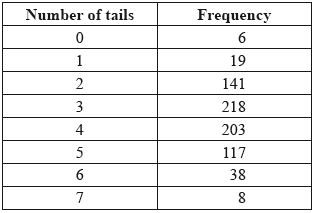
Explain what can be done with this data to decrease the probability of making a type I error.
(i) State the meaning of a type II error.
(ii) Write down how to proceed if it is required to decrease the probability of making both a type I and type II error.
Markscheme
reduce the significance level (or equivalent statement) R2
[2 marks]
(i) accepting \({{\text{H}}_0}\) (or failing to reject \({{\text{H}}_0}\)) when it is false (or equivalent) A1
(ii) increase the number of trials A1
[2 marks]
Examiners report
It was disappointing to see that some candidates wrote incorrect hypotheses, eg ‘\({{\text{H}}_0}\): Data are binomial; \({{\text{H}}_1}\): Data are not binomial’ without specifying any parameters. Part (b) caused unexpected problems for many candidates who misunderstood the question and gave ‘increase the number of trials’ as their answer.
The random variable X has a binomial distribution with parameters \(n\) and \(p\).
Let \(U = nP\left( {1 - P} \right)\).
Show that \(P = \frac{X}{n}\) is an unbiased estimator of \(p\).
Show that \({\text{E}}\left( U \right) = \left( {n - 1} \right)p\left( {1 - p} \right)\).
Hence write down an unbiased estimator of Var(X).
Markscheme
\({\text{E}}\left( P \right) = {\text{E}}\left( {\frac{X}{n}} \right) = \frac{1}{n}{\text{E}}\left( X \right)\) M1
\( = \frac{1}{n}\left( {np} \right) = p\) A1
so P is an unbiased estimator of \(p\) AG
[2 marks]
\({\text{E}}\left( {nP\left( {1 - P} \right)} \right) = {\text{E}}\left( {n\left( {\frac{X}{n}} \right)\left( {1 - \frac{X}{n}} \right)} \right)\)
\( = {\text{E}}\left( X \right) = \frac{1}{n}{\text{E}}\left( {{X^2}} \right)\) M1A1
use of \({\text{E}}\left( {{X^2}} \right) = {\text{Var}}\left( X \right) + {\left( {{\text{E}}\left( X \right)} \right)^2}\) M1
Note: Allow candidates to work with P rather than X for the above 3 marks.
\( = np - \frac{1}{n}\left( {np\left( {1 - p} \right) + {{\left( {np} \right)}^2}} \right)\) A1
\( = np - p\left( {1 - p} \right) - n{p^2}\)
\( = np\left( {1 - p} \right) - p\left( {1 - p} \right)\) A1
Note: Award A1 for the factor of \(\left( {1 - p} \right)\).
\( = \left( {n - 1} \right)p\left( {1 - p} \right)\) AG
[5 marks]
an unbiased estimator is \(\frac{{{n^2}P\left( {1 - P} \right)}}{{n - 1}}\left( { = \frac{{nU}}{{n - 1}}} \right)\) A1
[1 mark]
Examiners report
Two students are selected at random from a large school with equal numbers of boys and girls. The boys’ heights are normally distributed with mean \(178\) cm and standard deviation \(5.2\) cm, and the girls’ heights are normally distributed with mean \(169\) cm and standard deviation \(5.4\) cm.
Calculate the probability that the taller of the two students selected is a boy.
Markscheme
let \(X\) denote boys’ height and \(Y\) denote girls’ height
if \(BB,{\text{ P(taller is boy)}} = 1\) (A1)
if \(GG,{\text{ P(taller is boy)}} = 0\) (A1)
if \(BG\) or \(GB\):
consider \(X - Y\) (M1)
\(E(X - Y) = 178 - 169 = 9\) A1
\({\text{Var}}(X - Y) = {5.2^2} + {5.4^2}\;\;\;( = 56.2)\) (M1)A1
\({\text{P}}(X - Y > 0) = 0.885\) A1
answer is \(\frac{1}{4} \times 1 + \frac{1}{2} \times 0.885 = 0.693\) (M1)A1
[9 marks]
Examiners report
A hospital specializes in treating overweight patients. These patients have weights that are independently, normally distributed with mean 200 kg and standard deviation 15 kg. The elevator in the hospital will break if the total weight of people inside it exceeds 1150 kg. Six patients enter the elevator.
Find the probability that the elevator breaks.
Markscheme
let \(W = \sum\limits_{i = 1}^6 {{w_i}} \) (M1)
\({w_i}{\text{ is N}}(200,{\text{ 1}}{{\text{5}}^2})\)
\({\text{E}}(W) = \sum\limits_{i = 1}^6 {{\text{E}}({w_i}) = 6 \times 200 = 1200} \) A1
\({\text{Var}}(W) = \sum\limits_{i = 1}^6 {{\text{Var}}({w_i}) = 6 \times {{15}^2} = 1350} \) A2
\(W{\text{ is N}}(1200,{\text{ 1350}})\) (M1)
\({\text{P}}(W > 1150) = 0.913\) by GDC A1A1
Note: Using 6 times the mean or a lower bound for the mean are acceptable methods.
[7 marks]
Examiners report
Candidates will often be asked to solve these problems that test if they can distinguish between a number of individuals and a number of copies. The wording of the question was designed to make the difference clear. If candidates wrote \({w_1} + \ldots + {w_6}\) in (a) and 12w in (b), they usually went on to gain full marks.
Eleven students who had under-performed in a philosophy practice examination were given extra tuition before their final examination. The differences between their final examination marks and their practice examination marks were
\[10,{\text{ }} - 1,{\text{ }}6,{\text{ }}7,{\text{ }} - 5,{\text{ }} - 5,{\text{ }}2,{\text{ }} - 3,{\text{ }}8,{\text{ }}9,{\text{ }} - 2.\]
Assume that these differences form a random sample from a normal distribution with mean \(\mu \) and variance \({\sigma ^2}\).
Determine unbiased estimates of \(\mu \) and \({\sigma ^2}\).
(i) State suitable hypotheses to test the claim that extra tuition improves examination marks.
(ii) Calculate the \(p\)-value of the sample.
(iii) Determine whether or not the above claim is supported at the \(5\% \) significance level.
Markscheme
unbiased estimate of \(\mu \) is \(2.36(36 \ldots )\;\;\;(26/11)\) (M1)A1
unbiased estimate of \({\sigma ^2}\) is \(33.65(45 \ldots ) = ({5.801^2})\;\;\;(1851/55)\) (M1)A1
Note: Accept any answer that rounds correctly to \(3\) significant figures.
Note: Award M1A0 for any unbiased estimate of \({\sigma ^2}\) that rounds to \(5.80\).
[4 marks]
(i) \({{\text{H}}_0}:\mu = 0;{\text{ }}{{\text{H}}_1}:\mu > 0\) A1A1
Note: Award A1A0 if an inappropriate symbol is used for the mean, eg, \(r\), \({\rm{\bar d}}\).
(ii) attempt to use t-test (M1)
\(t = 1.35\) (A1)
\({\text{DF}} = 10\) (A1)
\(p\)-value \( = 0.103\) A1
Note: Accept any answer that rounds correctly to \(3\) significant figures.
(iii) \(0.103 > 0.05\) A1
there is insufficient evidence at the \(5\% \) level to support the claim (that extra tuition improves examination marks)
OR
the claim (that extra tuition improves examination marks) is not supported at the \(5\% \) level (or equivalent statement) R1
Note: Follow through the candidate’s \(p\)-value.
Note: Do not award R1 for Accept \({{\text{H}}_0}\) or Reject \({{\text{H}}_1}\).
[8 marks]
Total [12 marks]
Examiners report
Almost every candidate gave the correct estimate of the mean but some chose the wrong variance from their calculators to estimate \({\sigma ^2}\). In (b)(i), the hypotheses were sometimes incorrectly written, usually with an incorrect symbol instead of \(\mu \), for example \(d\), \(\bar x\) and ‘mean’ were seen. Many candidates failed to make efficient use of their calculators in (b)(ii). The intention of the question was that candidates should simply input the data into their calculators and use the software to give the p-value. Instead, many candidates found the p-value by first evaluating \(t\) using the appropriate formula. This was a time consuming process and it gave opportunity for error. In (b)(iii), candidates were expected to refer to the claim so that the answers ‘Accept \({H_0}\)’ or ‘Reject \({H_1}\)’ were not accepted.
Almost every candidate gave the correct estimate of the mean but some chose the wrong variance from their calculators to estimate \({\sigma ^2}\). In (b)(i), the hypotheses were sometimes incorrectly written, usually with an incorrect symbol instead of \(\mu \), for example \(d\), \(\bar x\) and ‘mean’ were seen. Many candidates failed to make efficient use of their calculators in (b)(ii). The intention of the question was that candidates should simply input the data into their calculators and use the software to give the \(p\)-value. Instead, many candidates found the \(p\)-value by first evaluating \(t\) using the appropriate formula. This was a time consuming process and it gave opportunity for error. In (b)(iii), candidates were expected to refer to the claim so that the answers ‘Accept \({H_0}\)’ or ‘Reject \({H_1}\)’ were not accepted.
Two species of plant, \(A\) and \(B\), are identical in appearance though it is known that the mean length of leaves from a plant of species \(A\) is \(5.2\) cm, whereas the mean length of leaves from a plant of species \(B\) is \(4.6\) cm. Both lengths can be modelled by normal distributions with standard deviation \(1.2\) cm.
In order to test whether a particular plant is from species \(A\) or species \(B\), \(16\) leaves are collected at random from the plant. The length, \(x\), of each leaf is measured and the mean length evaluated. A one-tailed test of the sample mean, \(\bar X\), is then performed at the \(5\% \) level, with the hypotheses: \({H_0}:\mu = 5.2\) and \({H_1}:\mu < 5.2\).
Find the critical region for this test.
It is now known that in the area in which the plant was found \(90\% \) of all the plants are of species \(A\) and \(10\% \) are of species \(B\).
Find the probability that \(\bar X\) will fall within the critical region of the test.
If, having done the test, the sample mean is found to lie within the critical region, find the probability that the leaves came from a plant of species \(A\).
Markscheme
\(\bar X \sim N\left( {5.2,{\text{ }}\frac{{{{1.2}^2}}}{{16}}} \right)\) (M1)
critical value is \(5.2 - 1.64485 \ldots \times \frac{{1.2}}{4} = 4.70654 \ldots \) (A1)
critical region is \(] - \infty ,{\text{ }}4.71]\) A1
Note: Allow follow through for the final A1 from their critical value.
Note: Follow through previous values in (b), (c) and (d).
[3 marks]
\(0.9 \times 0.05 + 0.1 \times (1 - 0.361 \ldots ) = 0.108875997 \ldots = 0.109\) M1A1
Note: Award M1 for a weighted average of probabilities with weights \(0.1,0.9\).
[2 marks]
attempt to use conditional probability formula M1
\(\frac{{0.9 \times 0.05}}{{0.108875997 \ldots }}\) (A1)
\( = 0.41334 \ldots = 0.413\) A1
[3 marks]
Total [10 marks]
Examiners report
Solutions to this question were generally disappointing.
In (a), the standard error of the mean was often taken to be \(\sigma (1.2)\) instead of \(\frac{\sigma }{{\sqrt n }}(0.3)\) and the solution sometimes ended with the critical value without the critical region being given.
In (c), the question was often misunderstood with candidates finding the weighted mean of the two means, ie \(0.9 \times 5.2 + 0.1 \times 4.6 = 5.14\) instead of the weighted mean of two probabilities.
Without having the solution to (c), part (d) was inaccessible to most of the candidates so that very few correct solutions were seen.
A factory makes wine glasses. The manager claims that on average 2 % of the glasses are imperfect. A random sample of 200 glasses is taken and 8 of these are found to be imperfect.
Test the manager’s claim at a 1 % level of significance using a one-tailed test.
Markscheme
Let X denote the number of imperfect glasses in the sample (M1)
For recognising binomial or proportion or Poisson A1
(\(X \sim {\text{B}}(200,{\text{ }}p)\) where p-value is the probability of a glass being imperfect)
Let \({{\text{H}}_0}:p{\text{-value}} = 0.02{\text{ and }}{{\text{H}}_1}:p{\text{-value}} > 0.02\) A1A1
EITHER
p-value = 0.0493 A2
Using the binomial distribution \(p{\text{-value}} = 0.0493 > 0.01{\text{ we accept }}{{\text{H}}_0}\) R1
OR
p-value = 0.0511 A2
Using the Poisson approximation to the binomial distribution since \(p{\text{-value}} = 0.0511 > 0.01{\text{ we accept }}{{\text{H}}_0}\) R1
OR
p-value = 0.0217 A2
Using the one proportion z-test since \(p{\text{-value}} = 0.0217 > 0.01{\text{ we accept }}{{\text{H}}_0}\) R1
Note: Use of critical values is acceptable.
[7 marks]
Examiners report
Many candidates used a t-test on this question. This was possibly because the sample was large enough to approximate normality of a proportion. The need to use a one-tailed test was often missed. When using the z-test of proportions p = 0.04 was often used instead of p = 0.02 . Not many candidates used the binomial distribution.
Ten friends try a diet which is claimed to reduce weight. They each weigh themselves before starting the diet, and after a month on the diet, with the following results.

Determine unbiased estimates of the mean and variance of the loss in weight achieved over the month by people using this diet.
(i) State suitable hypotheses for testing whether or not this diet causes a mean loss in weight.
(ii) Determine the value of a suitable statistic for testing your hypotheses.
(iii) Find the 1 % critical value for your statistic and state your conclusion.
Markscheme
the weight losses are
2.2\(\,\,\,\,\,\)3.5\(\,\,\,\,\,\)4.3\(\,\,\,\,\,\)–0.5\(\,\,\,\,\,\)4.2\(\,\,\,\,\,\)–0.2\(\,\,\,\,\,\)2.5\(\,\,\,\,\,\)2.7\(\,\,\,\,\,\)0.1\(\,\,\,\,\,\)–0.7 (M1)(A1)
\(\sum {x = 18.1} \), \(\sum {{x^2} = 67.55} \)
UE of mean = 1.81 A1
UE of variance \( = \frac{{67.55}}{9} - \frac{{{{18.1}^2}}}{{90}} = 3.87\) (M1)A1
Note: Accept weight losses as positive or negative. Accept unbiased estimate of mean as positive or negative.
Note: Award M1A0 for 1.97 as UE of variance.
[5 marks]
(i) \({H_0}:{\mu _d} = 0\) versus \({H_1}:{\mu _d} > 0\) A1
Note: Accept any symbol for \({\mu _d}\)
(ii) using t test (M1)
\(t = \frac{{1.81}}{{\sqrt {\frac{{3.87}}{{10}}} }} = 2.91\) A1
(iii) DF = 9 (A1)
Note: Award this (A1) if the p-value is given as 0.00864
1% critical value = 2.82 A1
accept \({H_1}\) R1
Note: Allow FT on final R1.
[6 marks]
Examiners report
In (a), most candidates gave a correct estimate for the mean but the variance estimate was often incorrect. Some candidates who use their GDC seem to be unable to obtain the unbiased variance estimate from the numbers on the screen. The way to proceed, of course, is to realise that the larger of the two ‘standard deviations’ on offer is the square root of the unbiased estimate so that its square gives the required result. In (b), most candidates realised that the t-distribution should be used although many were awarded an arithmetic penalty for giving either t = 2.911 or the critical value = 2.821. Some candidates who used the p-value method to reach a conclusion lost a mark by omitting to give the critical value. Many candidates found part (c) difficult and although they were able to obtain t = 2.49…, they were then unable to continue to obtain the confidence interval.
In (a), most candidates gave a correct estimate for the mean but the variance estimate was often incorrect. Some candidates who use their GDC seem to be unable to obtain the unbiased variance estimate from the numbers on the screen. The way to proceed, of course, is to realise that the larger of the two ‘standard deviations’ on offer is the square root of the unbiased estimate so that its square gives the required result. In (b), most candidates realised that the t-distribution should be used although many were awarded an arithmetic penalty for giving either t = 2.911 or the critical value = 2.821. Some candidates who used the p-value method to reach a conclusion lost a mark by omitting to give the critical value. Many candidates found part (c) difficult and although they were able to obtain t = 2.49…, they were then unable to continue to obtain the confidence interval.
The owner of a factory is asked to produce bricks of weight 2.2 kg. The quality control manager wishes to test whether or not, on a particular day, the mean weight of bricks being produced is 2.2 kg.
He therefore collects a random sample of 20 of these bricks and determines the weight, \(x\) kg, of each brick. He produces the following summary statistics.
\[\sum {x = 42.0,{\text{ }}\sum {{x^2} = 89.2} } \]
State hypotheses to enable the quality control manager to test the mean weight using a two-tailed test.
(i) Calculate unbiased estimates of the mean and the variance of the weights of the bricks being produced.
(ii) Assuming that the weights of the bricks are normally distributed, determine the \(p\)-value of the above results and state the conclusion in context using a 5% significance level.
The owner is more familiar with using confidence intervals. Determine a 95% confidence interval for the mean weight of bricks produced on that particular day.
Markscheme
\({H_0}:{\text{ }}\mu = 2.2;{\text{ }}{H_1}:{\text{ }}\mu \ne 2.2\) A1A1
[2 marks]
(i) UE of mean \( = \frac{{42.0}}{{20}}{\text{ = }}2.1\) A1
UE of variance \( = \frac{{89.2}}{{19}} - \frac{{20 \times {{2.1}^2}}}{{19}} = 0.0526{\text{ }}\left( {\frac{1}{{19}}} \right)\) (M1)A1
Note: Award (M0) for division by 20 where there is no subsequent use of \(\frac{{20}}{{19}}\).
(ii)
\(t = - 1.95\) (A1)
\({\text{DF}} = 19\) (A1)
\(p - value = 0.0662\) A1
Note: Allow follow through from (b)(i). In particular, 0.05 for the variance gives \(t = - 2\) and \(p\)-value 0.0600.
accept \({H_0}\), or equivalent statement involving \({H_0}\) or \({H_1}\), indicating that the mean weight is 2.2kg R1
Note: Follow through the candidate’s \(p\)-value.
[7 marks]
\([1.99,{\text{ }}2.21]\) A1A1
Note: Allow follow through from (b)(i). In particular, 0.05 for the variance gives \([2.00,{\text{ }}2.20]\).
[2 marks]
Examiners report
Most candidates stated the correct hypotheses in (a).
In (b)(i), the mean was invariably found correctly, although to find the variance estimate, quite a few candidates divided by 20 instead of 19. Incorrect variances were followed through in the next part of (b)(i). The \(t\)-test was generally well applied and the correct conclusion drawn. It was, however, surprising to note that many candidate used the appropriate formula to find the value of \(t\) and hence the \(p\)-value as opposed to using their GDC software.
Part (c) was generally well answered.
The continuous random variable \(X\) takes values in the interval \([0,{\text{ }}\theta ]\) and
\({\text{E}}(X) = \frac{\theta }{2}\) and \({\text{Var}}(X) = \frac{{{\theta ^2}}}{{24}}\).
To estimate the unknown parameter \(\theta \), a random sample of size \(n\) is obtained from the distribution of \(X\). The sample mean is denoted by \(\overline X \) and \(U = k\overline X\) is an unbiased estimator for \(\theta \).
Find the value of \(k\).
(i) Calculate an unbiased estimate for \(\theta \), using the random sample,
8.3, 4.2, 6.5, 10.3, 2.7, 1.2, 3.3, 4.3.
(ii) Explain briefly why this is not a good estimate for \(\theta \).
(i) Show that \({\text{Var}}(U) = \frac{{{\theta ^2}}}{{6n}}\).
(ii) Show that \({U^2}\) is not an unbiased estimator for \({\theta ^2}\).
(iii) Find an unbiased estimator for \({\theta ^2}\) in terms of \(U\) and \(n\).
Markscheme
\({\text{E}}(U) = k{\text{E}}(\overline X ) = k{\text{E}}(X)\) (M1)
\( = \frac{{k\theta }}{2}\) (A1)
unbiased when \(k = 2\) A1
[3 marks]
(i) for the data, \(\Sigma x = 40.8\) (A1)
\( \Rightarrow \bar x = 5.1\) (A1)
so that unbiased estimate for \(\theta = 10.2\) A1
(ii) this is impossible because of the sample value 10.3 R1
[4 marks]
(i) \({\text{Var}}(U) = 4 \times {\text{Var}}(\bar X)\) (M1)
\( = 4 \times \frac{{{\theta ^2}}}{{24n}}\) A1
\( = \frac{{{\theta ^2}}}{{6n}}\) AG
(ii) \({\text{E}}({U^2}) = {\text{Var}}(U) + {\left( {{\text{E}}(U)} \right)^2}\) M1
\( = \frac{{{\theta ^2}}}{{6n}} + {\theta ^2}\) A1
\({\text{E}}({U^2}) \ne {\theta ^2}\) R1
so not unbiased AG
(iii) \({\text{E}}({U^2}) = \frac{{{\theta ^2}}}{{6n}}(1 + 6n)\) (A1)
\({\text{E}}\left( {\left( {\frac{{6n}}{{1 + 6n}}} \right){U^2}} \right) = {\theta ^2}\) (A1)
therefore \(\left( {\left( {\frac{{6n}}{{1 + 6n}}} \right){U^2}} \right)\) is an unbiased estimator for \({\theta ^2}\) A1
[8 marks]
Examiners report
Solutions to (a) were often disappointing with some candidates seeming to be confused by the notation used.
In (b)(i), many candidates evaluated the sample mean as 5.1 but some failed to convert this to the estimate 10.2 even if they had correctly found the value of \(k\).
In (b)(ii), very few candidates realised that \(\theta = 10.2\) was not a feasible estimate when one of the sample values was 10.3.
Solutions to (c) were generally poor.
In (c)(i), many good answers were seen although some candidates failed to take account of the difference between \({\text{Var}}(X)\) and \({\text{Var}}(\bar X)\).
In (c)(ii), many candidates thought that \({\text{E}}({\bar X^2}) = {\left[ {{\text{E}}(\bar X)} \right]^2}\) although this had the unfortunate consequence of showing that \({U^2}\) is an unbiased estimator for \({\theta ^2}\). Few candidates realized that an expression for \({\text{E}}({U^2})\) could be found by considering the standard result that \({\text{Var}}(U) = {\text{E}}({U^2}) - {\left[ {{\text{E}}(U)} \right]^2}\) or the equivalent expression for \({\text{Var}}(\bar X)\). Part (c)(iii) was inaccessible to candidates who were unable to solve (ii).
(a) After a chemical spillage at sea, a scientist measures the amount, x units, of the chemical in the water at 15 randomly chosen sites. The results are summarised in the form \(\sum {x = 18} \) and \(\sum {{x^2} = 28.94} \). Before the spillage occurred the mean level of the chemical in the water was 1.1. Test at the 5 % significance level the hypothesis that there has been an increase in the amount of the chemical in the water.
(b) Six months later the scientist returns and finds that the mean amount of the chemical in the water at the 15 randomly chosen sites is 1.18. Assuming that this sample came from a normal population with variance 0.0256, find a 90 % confidence interval for the mean level of the chemical.
Markscheme
(a) \(\bar x = \frac{{\sum x }}{n} = 1.2\) (A1)
\(s_{n - 1}^2 = 0.524 \ldots \) (A1)
it is a one tailed test
\({{\text{H}}_0}:\mu = 1.1,{\text{ }}{{\text{H}}_1}:\mu > 1.1\) A1
EITHER
\(t = \frac{{1.2 - 1.1}}{{\sqrt {\frac{{0.524 \ldots }}{{15}}} }} = 0.535\) (M1) A1
\(v = 14\) (A1)
\({t_{crit}} = 1.761\) A1
since \(0.535 < {t_{crit}}\) we accept \({{\text{H}}_0}\) that there is no increase in the amount of the chemical R1
OR
\(p = 0.301\) A4
since \(p > 0.05\) we accept \({{\text{H}}_0}\) that there is no increase in the amount of the chemical R1
[8 marks]
(b) 90 % confidence interval \( = 1.18 \pm 1.645\sqrt {\frac{{0.0256}}{{15}}} \) (M1)A1A1A1
\( = [1.11,{\text{ }}1.25]\) A1 N5
[5 marks]
Total [13 marks]
Examiners report
This question also proved accessible to a majority of candidates with many wholly correct or nearly wholly correct answers seen. A few candidates did not recognise that part (a) was a t-distribution and part (b) was a Normal distribution, but most recognised the difference. Many candidates received an accuracy penalty on this question for not giving the final answer to part (b) to 3 significant figures.
A shopper buys 12 apples from a market stall and weighs them with the following results (in grams).
117, 124, 129, 118, 124, 116, 121, 126, 118, 121, 122, 129
You may assume that this is a random sample from a normal distribution with mean \(\mu \) and variance \({\sigma ^2}\).
Determine unbiased estimates of \(\mu \) and \({\sigma ^2}\).
Determine a 99 % confidence interval for \(\mu \) .
The stallholder claims that the mean weight of apples is 125 grams but the shopper claims that the mean is less than this.
(i) State suitable hypotheses for testing these claims.
(ii) Calculate the p-value of the above sample.
(iii) Giving a reason, state which claim is supported by your p-value using a 5 % significance level.
Markscheme
unbiased estimate of \(\mu = 122\) A1
unbiased estimate of \({\sigma ^2} = 4.4406{ \ldots ^2} = 19.7\) (M1)A1
Note: Award (M1)A0 for 4.44.
[3 marks]
the 99 % confidence interval for \(\mu \) is [118, 126] A1A1
[2 marks]
(i) \({{\text{H}}_0}:\mu = 125;{\text{ }}{{\text{H}}_1}:\mu < 125\) A1
(ii) p-value = 0.0220 A2
(iii) the shopper’s claim is supported because \(0.0220 < 0.05\) A1R1
[5 marks]
Examiners report
Engine oil is sold in cans of two capacities, large and small. The amount, in millilitres, in each can, is normally distributed according to Large \( \sim {\text{N}}(5000,{\text{ }}40)\) and Small \( \sim {\text{N}}(1000,{\text{ }}25)\).
A large can is selected at random. Find the probability that the can contains at least \(4995\) millilitres of oil.
A large can and a small can are selected at random. Find the probability that the large can contains at least \(30\) milliliters more than five times the amount contained in the small can.
A large can and five small cans are selected at random. Find the probability that the large can contains at least \(30\) milliliters less than the total amount contained in the small cans.
Markscheme
\({\text{P}}(L \ge 4995) = 0.785\) (M1)A1
Note: Accept any answer that rounds correctly to \(0.79\).
Award M1A0 for \(0.78\).
Note: Award M1A0 for any answer that rounds to \(0.55\) obtained by taking \({\text{SD}} = 40\).
[2 marks]
we are given that \(L \sim {\text{N}}(5000,{\text{ }}40)\) and \(S \sim {\text{N}}(1000,{\text{ }}25)\)
consider \(X = L - 5S\) (ignore \( \pm 30\)) (M1)
\({\text{E}}(X) = 0\) (\( \pm 30\) consistent with line above) A1
\({\text{Var}}(X) = {\text{Var}}(L) + 25{\text{Var}}(S) = 40 + 625 = 665\) (M1)A1
require \({\text{P}}(X \ge 30)\;\;\;({\text{or P}}(X \ge 0){\text{ if }} - 30{\text{ above}})\) (M1)
obtain \(0.122\) A1
Note: Accept any answer that rounds correctly to \(2\) significant figures.
[6 marks]
consider \(Y = L - ({S_1} + {S_2} + {S_3} + {S_4} + {S_5})\) (ignore \( \pm 30\)) (M1)
\({\text{E}}(Y) = 0\) (\( \pm 30\) consistent with line above) A1
\({\text{Var}}(Y) = 40 + 5 \times 25 = 165\) A1
require \({\text{P}}(Y \le - 30){\text{ (or P}}(Y \le 0){\text{ if }} + 30{\text{ above)}}\) (M1)
obtain \(0.00976\) A1
Note: Accept any answer that rounds correctly to \(2\) significant figures.
Note: Condone the notation \(Y = L - 5S\) if the variance is correct.
[5 marks]
Total [13 marks]
Examiners report
Most candidates solved (a) correctly. In (b) and (c), however, many candidates made the usual error of confusing \(\sum\limits_{i = 1}^n {{X_i}} \) and \(nX\). Indeed some candidates even use the second expression to mean the first. This error leads to an incorrect variance and of course an incorrect answer. Some candidates had difficulty in converting the verbal statements into the correct probability statements, particularly in (c).
Most candidates solved (a) correctly. In (b) and (c), however, many candidates made the usual error of confusing \(\sum\limits_{i = 1}^n {{X_i}} \) and \(nX\). Indeed some candidates even use the second expression to mean the first. This error leads to an incorrect variance and of course an incorrect answer. Some candidates had difficulty in converting the verbal statements into the correct probability statements, particularly in (c).
Most candidates solved (a) correctly. In (b) and (c), however, many candidates made the usual error of confusing \(\sum\limits_{i = 1}^n {{X_i}} \) and \(nX\). Indeed some candidates even use the second expression to mean the first. This error leads to an incorrect variance and of course an incorrect answer. Some candidates had difficulty in converting the verbal statements into the correct probability statements, particularly in (c).
The number of machine breakdowns occurring in a day in a certain factory may be assumed to follow a Poisson distribution with mean \(\mu \). The value of \(\mu \) is known, from past experience, to be 1.2. In an attempt to reduce the value of \(\mu \), all the machines are fitted with new control units. To investigate whether or not this reduces the value of \(\mu \), the total number of breakdowns, x, occurring during a 30-day period following the installation of these new units is recorded.
State suitable hypotheses for this investigation.
It is decided to define the critical region by \(x \leqslant 25\).
(i) Calculate the significance level.
(ii) Assuming that the value of \(\mu \) was actually reduced to 0.75, determine the probability of a Type II error.
Markscheme
\({{\text{H}}_0}:\mu = 1.2\); \({{\text{H}}_1}:\mu < 1.2\) A1
Note: Accept “ \({{\text{H}}_0}:\) (\(30\)-day) mean \( = 36\); \({{\text{H}}_1}:\) (\(30\)-day) mean \( = 36\) ”.
[1 mark]
(i) let X denote the number of breakdowns in 30 days
then under \({{\text{H}}_0}\) , \(E(X) = 36\) (A1)
\({\text{sig level}} = {\text{P}}(X \leqslant 25|{\text{mean}} = 36)\) (M1)(A1)
= 0.0345 (3.45%) A1
Note: Accept any answer that rounds to 0.035 (3.5%) .
Note: Do not accept the use of a normal approximation.
(ii) under \({{\text{H}}_1}\), \(E(X) = 22.5\) (A1)
\(P{\text{(Type II error)}} = P(X \geqslant 26|{\text{mean}} = 22.5)\) (M1)(A1)
= 0.257 A1
Note: Accept any answer that rounds to 0.26.
Note: Do not accept the use of a normal approximation.
[8 marks]
Examiners report
This question was well answered by many candidates. The most common error was to attempt to use a normal approximation to find approximate probabilities instead of the Poisson distribution to find the exact probabilities. Some candidates appeared not to be familiar with the term ‘Type II error probability’ which made (b)(ii) inaccessible. Another fairly common error was to believe that the complement of \(x \leqslant 25\) is \(x \geqslant 25\).
This question was well answered by many candidates. The most common error was to attempt to use a normal approximation to find approximate probabilities instead of the Poisson distribution to find the exact probabilities. Some candidates appeared not to be familiar with the term ‘Type II error probability’ which made (b)(ii) inaccessible. Another fairly common error was to believe that the complement of \(x \leqslant 25\) is \(x \geqslant 25\).
Determine the probability generating function for \(X \sim {\text{B}}(1,{\text{ }}p)\).
Explain why the probability generating function for \({\text{B}}(n,{\text{ }}p)\) is a polynomial of degree \(n\).
Two independent random variables \({X_1}\) and \({X_2}\) are such that \({X_1} \sim {\text{B}}(1,{\text{ }}{p_1})\) and \({X_2} \sim {\text{B}}(1,{\text{ }}{p_2})\). Prove that if \({X_1} + {X_2}\) has a binomial distribution then \({p_1} = {p_2}\).
Markscheme
\({\text{P}}(X = 0) = 1 - p( = q);{\text{ P}}(X = 1) = p\) (M1)(A1)
\({{\text{G}}_x}(t) = \sum\limits_r {{\text{P}}(X = r){t^r}\;\;\;} \)(or writing out term by term) M1
\( = q + pt\) A1
[4 marks]
METHOD 1
\(PGF\) for \(B(n,{\text{ }}p)\) is \({(q + pt)^n}\) R1
which is a polynomial of degree \(n\) R1
METHOD 2
in \(n\) independent trials, it is not possible to obtain more than \(n\) successes (or equivalent, eg, \({\text{P}}(X > n) = 0\)) R1
so \({a_r} = 0\) for \(r > n\) R1
[2 marks]
let \(Y = {X_1} + {X_2}\)
\({G_Y}(t) = ({q_1} + {p_1}t)({q_2} + {p_2}t)\) A1
\({G_Y}(t)\) has degree two, so if \(Y\) is binomial then
\(Y \sim {\text{B}}(2,{\text{ }}p)\) for some \(p\) R1
\({(q + pt)^2} = ({q_1} + {p_1}t)({q_2} + {p_2}t)\) A1
Note: The \(LHS\) could be seen as \({q^2} + 2pqt + {p^2}{t^2}\).
METHOD 1
by considering the roots of both sides, \(\frac{{{q_1}}}{{{p_1}}} = \frac{{{q_2}}}{{{p_2}}}\) M1
\(\frac{{1 - {p_1}}}{{{p_1}}} = \frac{{1 - {p_2}}}{{{p_2}}}\) A1
so \({p_1} = {p_2}\) AG
METHOD 2
equating coefficients,
\({p_1}{p_2} = {p^2},{\text{ }}{q_1}{q_2} = {q^2}{\text{ or }}(1 - {p_1})(1 - {p_2}) = {(1 - p)^2}\) M1
expanding,
\({p_1} + {p_2} = 2p\) so \({p_1},{\text{ }}{p_2}\) are the roots of \({x^2} - 2px + {p^2} = 0\) A1
so \({p_1} = {p_2}\) AG
[5 marks]
Total [11 marks]
Examiners report
Solutions to (a) were often disappointing with some candidates simply writing down the answer. A common error was to forget the possibility of \(X\) being zero so that \(G(t) = pt\) was often seen.
Explanations in (b) were often poor, again indicating a lack of ability to give a verbal explanation.
Very few complete solutions to (c) were seen with few candidates even reaching the result that \(({q_1} + {p_1}t)({q_2} + {p_2}t)\) must equal \({(q + pt)^2}\) for some \(p\).
Ahmed and Brian live in the same house. Ahmed always walks to school and Brian always cycles to school. The times taken to travel to school may be assumed to be independent and normally distributed. The mean and the standard deviation for these times are shown in the table below.

(a) Find the probability that on a particular day Ahmed takes more than 35 minutes to walk to school.
(b) Brian cycles to school on five successive mornings. Find the probability that the total time taken is less than 70 minutes.
(c) Find the probability that, on a particular day, the time taken by Ahmed to walk to school is more than twice the time taken by Brian to cycle to school.
Markscheme
(a) \(A \sim {\text{N}}(30,{\text{ }}{3^2})\)
\({\text{P}}(A > 35) = 0.0478\) (M1)A1
[2 marks]
(b) let \(X = {B_1} + {B_2} + {B_3} + {B_4} + {B_5}\)
\({\text{E}}(X) = 5{\text{E}}(B) = 60\) A1
\({\text{Var}}(X) = 5{\text{Var}}(B) = 20\) (M1)A1
\({\text{P}}(X < 70) = 0.987\) A1
[4 marks]
(c) let \(Y = A - 2B\) (M1)
\({\text{E}}(Y) = {\text{E}}(A) - 2{\text{E}}(B) = 6\) A1
\({\text{Var}}(Y) = {\text{Var}}(A) + 4{\text{Var}}(B) = 25\) (M1)A1
\({\text{P}}(Y > 0) = 0.885\) A1
[5 marks]
Total [11 marks]
Examiners report
Most candidates were able to access this question, but weaker candidates did not always realise that parts (b) and (c) were testing different things. Part (b) proved the hardest with a number of candidates not understanding how to find the variance of the sum of variables.
A manufacturer of stopwatches employs a large number of people to time the winner of a \(100\) metre sprint. It is believed that if the true time of the winner is \(\mu \) seconds, the times recorded are normally distributed with mean \(\mu \) seconds and standard deviation \(0.03\) seconds.
The times, in seconds, recorded by six randomly chosen people are
\[9.765,{\text{ }}9.811,{\text{ }}9.783,{\text{ }}9.797,{\text{ }}9.804,{\text{ }}9.798.\]
Calculate a \(99\% \) confidence interval for \(\mu \). Give your answer correct to three decimal places.
Interpret the result found in (a).
Find the confidence level of the interval that corresponds to halving the width of the \(99\% \) confidence interval. Give your answer as a percentage to the nearest whole number.
Markscheme
the (unbiased) estimate of \(\mu \) is 9.793 (A1)
the \(99\% \) CI is \(9.793 \pm 2.576\frac{{0.03}}{{\sqrt 6 }}\) (M1)(A1)
\( = [9.761,{\text{ }}9.825]\) A1
Note: Accept \(9.762\) and \(9.824\).
[4 marks]
if this process is carried out a large number of times A1
(approximately) \(99\% \) of the intervals will contain \(\mu \) A1
Note: Award A1A1 for a consideration of any specific large value of times \((n \ge 100)\).
[2 marks]
METHOD 1
If the interval is halved, \(2.576\) becomes \(1.288\) M1
normal tail probability corresponding to \(1.288 = 0.0988 \ldots \) A1
confidence level \( = 80\% \) A1
METHOD 2
half width \( = 0.5 \times 0.063\) or \(0.062\) or \(0.064 = 0.0315\) or \(0.031\) or \(0.032\) M1
\(\frac{{2z \times 0.03}}{{\sqrt 6 }} = 0.0315\) or \(0.031\) or \(0.032\)
giving \(z = 1.285 \ldots \) or \(1.265 \ldots \) or \(1.306 \ldots \) A1
confidence level \( = 80\% \) or \(79\% \) or \(81\% \) A1
Note: Follow through values from (a).
[3 marks]
Total [9 marks]
Examiners report
The intention in (a) was that candidates should input the data into their calculators and use the software to give the confidence interval. However, as in Question 2, many candidates calculated the mean and variance by hand and used the appropriate formulae to determine the confidence limits. Again valuable time was used up and opportunity for error introduced.
Answers to (b) were extremely disappointing with the vast majority giving an incorrect interpretation of a confidence interval. The most common answer given was along the lines of ‘There is a 99% probability that the interval [9.761, 9.825] contains \(\mu \)’. This is incorrect since the interval and \(\mu \) are both constants; the statement that the interval [9.761, 9.825] contains \(\mu \) is either true or false, there is no question of probability being involved. Another common response was ‘I am 99% confident that the interval [9.761, 9.825] contains \(\mu \)’. This is unsatisfactory partly because 99% confident is really a euphemism for 99% probability and partly because it answers the question ‘What is a 99% confidence interval for \(\mu \)’ by simply rearranging the words without actually going anywhere. The expected answer was that if the sampling was carried out a large number of times, then approximately 99% of the calculated confidence intervals would contain \(\mu \). A more rigorous response would be that a 99% confidence interval for \(\mu \) is an observed value of a random interval which contains \(\mu \) with probability 0.99 just as the number \(\bar x\) is an observed value of the random variable \(\bar X\). The concept of a confidence interval is a difficult one at this level but confidence intervals are part of the programme and so therefore is their interpretation. In view of the widespread misunderstanding of confidence intervals, partial credit was given on this occasion for interpretations involving 99% probability or confidence but this will not be the case in future examinations.
Many candidates solved (c) correctly, mostly using Method 2 in the mark scheme.
A random variable \(X\) has a population mean \(\mu \).
Explain briefly the meaning of
(i) an estimator of \(\mu \);
(ii) an unbiased estimator of \(\mu \).
A random sample \({X_1},{\text{ }}{X_2},{\text{ }}{X_3}\) of three independent observations is taken from the distribution of \(X\).
An unbiased estimator of \(\mu ,{\text{ }}\mu \ne 0\), is given by \(U = \alpha {X_1} + \beta {X_2} + (\alpha - \beta ){X_3}\),
where \(\alpha ,{\text{ }}\beta \in \mathbb{R}\).
(i) Find the value of \(\alpha \).
(ii) Show that \({\text{Var}}(U) = {\sigma ^2}\left( {2{\beta ^2} - \beta + \frac{1}{2}} \right)\) where \({\sigma ^2} = {\text{Var}}(X)\).
(iii) Find the value of \(\beta \) which gives the most efficient estimator of \(\mu \) of this form.
(iv) Write down an expression for this estimator and determine its variance.
(v) Write down a more efficient estimator of \(\mu \) than the one found in (iv), justifying your answer.
Markscheme
(i) an estimator \(T\) is a formula (or statistic) that can be applied to the values in any sample, taken from \(X\) A1
to estimate the value of \(\mu \) A1
(ii) an estimator is unbiased if \({\text{E}}(T) = \mu \) A1
[3 marks]
(i) using linearity and the definition of an unbiased estimator M1
\(\mu = \alpha \mu + \beta \mu + (\alpha - \beta )\mu \) A1
obtain \(\alpha = \frac{1}{2}\) A1
(ii) attempt to compute \({\text{Var}}(U)\) using correct formula M1
\({\text{Var}}(U) = \frac{1}{4}{\sigma ^2} + {\beta ^2}{\sigma ^2} + {\left( {\frac{1}{2} - \beta } \right)^2}{\sigma ^2}\) A1
\({\text{Var}}(U) = {\sigma ^2}\left( {2{\beta ^2} - \beta + \frac{1}{2}} \right)\) AG
(iii) attempt to minimise quadratic in \(\beta \) (or equivalent) (M1)
\(\beta = \frac{1}{4}\) A1
(iv) \((U) = \frac{1}{2}{X_1} + \frac{1}{4}{X_2} + \frac{1}{4}{X_3}\) A1
\({\text{Var}}(U) = \frac{3}{8}{\sigma ^2}\) A1
(v) \(\frac{1}{3}{X_1} + \frac{1}{3}{X_2} + \frac{1}{3}{X_3}\) A1
\({\text{Var}}\left( {\frac{1}{3}{X_1} + \frac{1}{3}{X_2} + \frac{1}{3}{X_3}} \right) = \frac{3}{9}{\sigma ^2}\) A1
\( < {\text{Var}}(U)\) R1
Note: Accept \(\sum\limits_{i = 1}^3 {{\lambda _i}{X_i}} \) if \(\sum\limits_{i = 1}^3 {{\lambda _i} = 1} \) and \(\sum\limits_{i = 1}^3 {\lambda _i^2 < \frac{3}{8}} \) and follow through to the variance if this is the case.
[12 marks]
Total [15 marks]
Examiners report
In general, solutions to (a) were extremely disappointing with the vast majority unable to give correct explanations of estimators and unbiased estimators. Solutions to (b) were reasonably good in general, indicating perhaps that the poor explanations in (a) were due to an inability to explain what they know rather than a lack of understanding.
Solutions to (b) were reasonably good in general, indicating perhaps that the poor explanations in (a) were due to an inability to explain what they know rather than a lack of understanding.
A shop sells apples, pears and peaches. The weights, in grams, of these three types of fruit may be assumed to be normally distributed with means and standard deviations as given in the following table.

Alan buys 1 apple and 1 pear while Brian buys 1 peach. Calculate the probability that the combined weight of Alan’s apple and pear is greater than twice the weight of Brian’s peach.
Markscheme
let X, Y, Z denote respectively the weights, in grams, of a randomly chosen apple, pear, peach
then \(U = X + Y - 2Z{\text{ is N}}(115 + 110 - 2 \times 105,{\text{ }}{5^2} + {4^2} + {2^2} \times {3^2})\) (M1)(A1)(A1)
Note: Award M1 for attempted use of U.
i.e. N(15, 77) A1
we require
\({\text{P}}(X + Y > 2Z) = {\text{P}}(U > 0)\) M1A1
\( = 0.956\) A2
Note: Award M0A0A2 for 0.956 only.
[8 marks]
Examiners report
Solutions to this question again illustrated the fact that many candidates are unable to distinguish between nX and \(\sum\limits_{i = 1}^n {{X_i}} \) so that many candidates obtained an incorrect variance to evaluate the final probability.
A traffic radar records the speed, \(v\) kilometres per hour (\({\text{km}}\,{{\text{h}}^{-{\text{1}}}}\)), of cars on a section of a road.
The following table shows a summary of the results for a random sample of 1000 cars whose speeds were recorded on a given day.
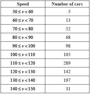
Using the data in the table,
(i) show that an estimate of the mean speed of the sample is 113.21 \({\text{km}}\,{{\text{h}}^{-{\text{1}}}}\);
(ii) find an estimate of the variance of the speed of the cars on this section of the road.
Find the 95% confidence interval, \(I\), for the mean speed.
Let \(J\) be the 90% confidence interval for the mean speed.
Without calculating \(J\), explain why \(J \subset I\).
Markscheme
(i) \(\bar v = \frac{1}{{1000}}(55 \times 5 + 65 \times 13 + \ldots + 145 \times 31)\) A1M1
Note: A1 for mid-points, M1 for use of the formula.
\( = \frac{{113\,210}}{{1000}} = 113.21\) AG
(ii) \({s^2} = \frac{{{{(55 - 113.21)}^2} \times 5 + {{(65 - 113.21)}^2} \times 13 + \ldots + {{(145 - 113.21)}^2} \times 31}}{{999}}\) (M1)
\( = \frac{{362\,295.9}}{{999}} = 362.6585 \ldots = 363\) A1
Note: Award A1 if answer rounds to 362 or 363.
Note: Condone division by 1000.
[4 marks]
\(\bar v \pm \frac{{{t_{0.025}} \times s}}{{\sqrt n }}\) (M1)
hence the confidence interval \(I = [112.028,{\text{ }}114.392]\) A1
Note: Accept answers which round to 112 and 114.
Note: Condone the use of \({z_{0.025}}\) for \({t_{0.025}}\) and \(\sigma \) for \(s\).
[2 marks]
less confidence implies narrower interval R2
Note: Accept equivalent statements or arguments having a meaningful diagram and/or relevant percentiles.
hence the confidence interval \(I\) at the 95% level contains the confidence interval \(J\) at the 90% level AG
[2 marks]
Examiners report
In (a)(i), the candidates were required to show that the estimate of the mean is 113.21 so that those who stated simply ‘Using my GDC, mean = 113.21’ were given no credit. Candidates were expected to indicate that the interval midpoints were used and to show the appropriate formula. In (a)(ii), division by either 999 or 1000 was accepted, partly because of the large sample size and partly because the question did not ask for an unbiased estimate of variance.
Solutions to (c) were often badly written, often quite difficult to understand exactly what was being stated.
As soon as Sarah misses a total of 4 lessons at her school an email is sent to her parents. The probability that she misses any particular lesson is constant with a value of \(\frac{1}{3}\). Her decision to attend a lesson is independent of her previous decisions.
(a) Find the probability that an email is sent to Sarah’s parents after the \({8^{{\text{th}}}}\) lesson that Sarah was scheduled to attend.
(b) If an email is sent to Sarah’s parents after the \({X^{{\text{th}}}}\) lesson that she was scheduled to attend, find \({\text{E}}(X)\).
(c) If after 6 of Sarah’s scheduled lessons we are told that she has missed exactly 2 lessons, find the probability that an email is sent to her parents after a total of 12 scheduled lessons.
(d) If we know that an email was sent to Sarah’s parents immediately after her \({6^{{\text{th}}}}\) scheduled lesson, find the probability that Sarah missed her \({2^{{\text{nd}}}}\) scheduled lesson.
Markscheme
(a) we are dealing with the Negative Binomial distribution: \({\text{NB}}\left( {4,\frac{1}{3}} \right)\) (M1)
let X be the number of scheduled lessons before the email is sent
\({\text{P}}(X = 8) = \left( {\begin{array}{*{20}{c}}
7 \\
3
\end{array}} \right){\left( {\frac{2}{3}} \right)^4}{\left( {\frac{1}{3}} \right)^4} = 0.0854\) (M1)A1
[3 marks]
(b) \({\text{E}}(X) = \frac{r}{p} = \frac{4}{{\frac{1}{3}}} = 12\) (M1)A1
[2 marks]
(c) we are asking for 2 missed lessons in the second 6 lessons, with the last lesson missed so this is \({\text{NB}}\left( {2,\frac{1}{3}} \right)\) (M1)
\({\text{P}}(X = 6) = \left( {\begin{array}{*{20}{c}}
5 \\
1
\end{array}} \right){\left( {\frac{2}{3}} \right)^4}{\left( {\frac{1}{3}} \right)^2} = 0.110\) (M1)A1
Note: Accept solutions laid out in terms of conditional probabilities.
[3 marks]
(d) EITHER
We know that she missed the \({6^{{\text{th}}}}\) lesson so she must have missed 3 from the first 5 lessons. All are equally likely so the probability that she missed the \({2^{{\text{nd}}}}\) lesson is \(\frac{3}{5}\). R1A1
OR
require \({\text{P(missed }}{{\text{2}}^{{\text{nd}}}}|X = 6) = \frac{{{\text{P(missed }}{{\text{2}}^{{\text{nd}}}}{\text{ and }}X = 6)}}{{{\text{P}}(X = 6)}}\) R1
\({\text{P(missed }}{{\text{2}}^{{\text{nd}}}}{\text{ and }}X = 6) = {\text{P(missed }}{{\text{2}}^{{\text{nd}}}}{\text{ and }}{{\text{6}}^{{\text{th}}}}{\text{ and 2 of remaining 4)}}\)
\[ = \frac{1}{3} \cdot \frac{1}{3} \cdot \left( {\begin{array}{*{20}{c}}
4 \\
2
\end{array}} \right){\left( {\frac{1}{3}} \right)^2}{\left( {\frac{2}{3}} \right)^2} = \frac{{24}}{{{3^6}}}\]
\({\text{P}}(X = 6) = \left( {\begin{array}{*{20}{c}}
5 \\
3
\end{array}} \right){\left( {\frac{1}{3}} \right)^4}{\left( {\frac{2}{3}} \right)^2} = \frac{{40}}{{{3^6}}}\)
so required probability is \(\frac{{24}}{{{3^6}}} \cdot \frac{{{3^6}}}{{40}} = \frac{3}{5}\) A1
[2 marks]
Total [10 marks]
Examiners report
Realising that this was a problem about the Negative Binomial distribution was the crucial thing to realise in this question. All parts of the syllabus do need to be covered.
The random variable X has a Poisson distribution with mean \(\mu \). The value of \(\mu \) is known to be either 1 or 2 so the following hypotheses are set up.
\[{{\text{H}}_0}:\mu = 1;{\text{ }}{{\text{H}}_1}:\mu = 2\]
A random sample \({x_1},{\text{ }}{x_2},{\text{ }} \ldots ,{\text{ }}{x_{10}}\) of 10 observations is taken from the distribution of X and the following critical region is defined.
\[\sum\limits_{i = 1}^{10} {{x_i} \geqslant 15} \]
Determine the probability of
(a) a Type I error;
(b) a Type II error.
Markscheme
(a) let \(T = \sum\limits_{i = 1}^{10} {{X_i}} \) so that T is Po(10) under \({{\text{H}}_0}\) (M1)
\({\text{P(Type I error)}} = {\text{P }}T \geqslant 15|\mu = 1\) M1A1
\( = 0.0835\) A2 N3
Note: Candidates who write the first line and only the correct answer award (M1)M0A0A2.
[5 marks]
(b) let \(T = \sum\limits_{i = 1}^{10} {{X_i}} \) so that T is Po(20) under \({{\text{H}}_1}\) (M1)
\({\text{P(Type II error)}} = {\text{P }}T \leqslant 14|\mu = 2\) M1A1
\( = 0.105\) A2 N3
Note: Candidates who write the first line and only the correct answer award (M1)M0A0A2.
Note: Award 5 marks to a candidate who confuses Type I and Type II errors and has both answers correct.
[5 marks]
Total [10 marks]
Examiners report
This question caused problems for many candidates and the solutions were often disappointing. Some candidates seemed to be unaware of the meaning of Type I and Type II errors. Others were unable to calculate the probabilities even when they knew what they represented. Candidates who used a normal approximation to obtain the probabilities were not given full credit – there seems little point in using an approximation when the exact value could be found.
In a game there are n players, where \(n > 2\) . Each player has a disc, one side of which is red and one side blue. When thrown, the disc is equally likely to show red or blue. All players throw their discs simultaneously. A player wins if his disc shows a different colour from all the other discs. Players throw repeatedly until one player wins.
Let X be the number of throws each player makes, up to and including the one on which the game is won.
(a) State the distribution of X .
(b) Find \({\text{P}}(X = x)\) in terms of n and x .
(c) Find \({\text{E}}(X)\) in terms of n .
(d) Given that n = 7 , find the least number, k , such that \({\text{P}}(X \leqslant k) > 0.5\) .
Markscheme
(a) geometric distribution A1
[1 mark]
(b) let R be the event throwing the disc and it landing on red and
let B be the event throwing the disc and it landing on blue
\({\text{P}}(X = 1) = p = {\text{P}}\left( {1B{\text{ and }}(n - 1)R{\text{ or }}1R{\text{ and }}(n - 1)B} \right)\) (M1)
\( = n \times \frac{1}{2} \times {\left( {\frac{1}{2}} \right)^{n - 1}} + n \times \frac{1}{2} \times {\left( {\frac{1}{2}} \right)^{n - 1}}\) (A1)
\( = \frac{n}{{{2^{n - 1}}}}\) A1
hence \({\text{P}}(X = x) = \frac{n}{{{2^{n - 1}}}}{\left( {1 - \frac{n}{{{2^{n - 1}}}}} \right)^{x - 1}},{\text{ }}(x \geqslant 1)\) A1
Notes: \(x \geqslant 1\) not required for final A1.
Allow FT for final A1.
[4 marks]
(c) \({\text{E}}(X) = \frac{1}{p}\)
\( = \frac{{{2^{n - 1}}}}{n}\) A1
[1 mark]
(d) when \(n = 7\) , \({\text{P}}(X = x) = {\left( {1 - \frac{7}{{64}}} \right)^{x - 1}} \times \frac{7}{{64}}\) (M1)
\( = \frac{7}{{64}} \times {\left( {\frac{{57}}{{64}}} \right)^{x - 1}}\)
\({\text{P}}(X \leqslant k) = \sum\limits_{x = 1}^k {\frac{7}{{64}} \times {{\left( {\frac{{57}}{{64}}} \right)}^{x - 1}}} \) (M1)(A1)
\( \Rightarrow \frac{7}{{64}} \times \frac{{1 - {{\left( {\frac{{57}}{{64}}} \right)}^k}}}{{1 - \frac{{57}}{{64}}}} > 0.5\) (M1)(A1)
\( \Rightarrow 1 - {\left( {\frac{{57}}{{64}}} \right)^k} > 0.5\)
\( \Rightarrow {\left( {\frac{{57}}{{64}}} \right)^k} < 0.5\)
\( \Rightarrow k > \frac{{\log 0.5}}{{\log \frac{{57}}{{64}}}}\) (M1)
\( \Rightarrow k > 5.98\) (A1)
\( \Rightarrow k = 6\) A1
Note: Tabular and other GDC methods are acceptable.
[8 marks]
Total [14 marks]
Examiners report
This question was found difficult by the majority of candidates and few fully correct answers were seen. Few candidates were able to find \({\text{P}}(X = x)\) in terms of n and x and many did not realise that the last part of the question required them to find the sum of a series. However, better candidates received over 75% of the marks because the answers could be followed through.
The length of time, T, in months, that a football manager stays in his job before he is removed can be approximately modelled by a normal distribution with population mean \(\mu \) and population variance \({\sigma ^2}\). An independent sample of five values of T is given below.
6.5, 12.4, 18.2, 3.7, 5.4
(a) Given that \({\sigma ^2} = 9\),
(i) use the above sample to find the 95 % confidence interval for \(\mu \), giving the bounds of the interval to two decimal places;
(ii) find the smallest number of values of T that would be required in a sample for the total width of the 90 % confidence interval for \(\mu \) to be less than 2 months.
(b) If the value of \({\sigma ^2}\) is unknown, use the above sample to find the 95 % confidence interval for \(\mu \), giving the bounds of the interval to two decimal places.
Markscheme
(a) (i) as \({\sigma ^2}\) is known \({\bar x}\) is \({\text{N}}\left( {\mu ,\frac{{{\sigma ^2}}}{n}} \right)\) (M1)
CI is \(\bar x - {z^ * }\frac{\sigma }{{\sqrt n }} < \mu < \bar x + {z^ * }\frac{\sigma }{{\sqrt n }}\) (M1)
\(\bar x = 9.24,{\text{ }}{z^ * } = 1.960\) for 95 % CI (A1)
CI is \(6.61 < \mu < 11.87\) by GDC A1A1
(ii) CI is \(\bar x - {z^ * }\frac{\sigma }{{\sqrt n }} < \mu < \bar x + {z^ * }\frac{\sigma }{{\sqrt n }}\)
require \(2 \times 1.645\frac{3}{{\sqrt n }} < 2\) R1A1
\(4.935 < \sqrt n \) (A1)
\(24.35 < n\) A1
so smallest value for n = 25 A1
Note: Accept use of table.
[10 marks]
(b) as \({\sigma ^2}\) is not known \({\bar x}\) has the t distribution with v = 4 (M1)(A1)
CI is \(\bar x - {t^ * }\frac{{{s_{n - 1}}}}{{\sqrt n }} < \mu < \bar x + {t^ * }\frac{{{s_{n - 1}}}}{{\sqrt n }}\)
\(\bar x = 9.24,{\text{ }}{s_{n - 1}} = 5.984,{\text{ }}{t^ * } = 2.776\) for 95 % CI (A1)
CI is \(1.81 < \mu < 16.67\) by GDC A1A1
[5 marks]
Total [15 marks]
Examiners report
The 2 confidence intervals were generally done well by using a calculator. Some marks were dropped by not giving the answers to 2 decimal places as required. Weak candidates did not realise that (b) was a t interval. Part (a) (ii) was not as well answered and often it was the first step that was the problem.
The random variable X is normally distributed with unknown mean \(\mu \) and unknown variance \({\sigma ^2}\) . A random sample of 10 observations on X was taken and the following 95 % confidence interval for \(\mu \) was correctly calculated as [4.35, 4.53] .
(a) Calculate an unbiased estimate for
(i) \(\mu \) ,
(ii) \({\sigma ^2}\) .
(b) The value of \(\mu \) is thought to be 4.5, so the following hypotheses are defined.\[{{\text{H}}_0}:\mu = 4.5;{\text{ }}{{\text{H}}_1}:\mu < 4.5\]
(i) Find the p-value of the observed sample mean.
(ii) State your conclusion if the significance level is
(a) 1 %,
(b) 10 %.
Markscheme
(a) (i) \(\bar x = \frac{{4.35 + 4.53}}{2} = 4.44\) (estimate of \(\mu \)) A2
(ii) Degrees of freedom = 9 (A1)
Critical value of t = 2.262 (A1)
\(2.262 \times \frac{s}{{\sqrt {10} }} = 0.09\) M1A1
\(s = 0.12582…\) (A1)
\({s^2} = 0.0158\) (estimate of \({\sigma ^2}\)) A1
[8 marks]
(b) (i) Using t test (M1)
\(t = \frac{{4.44 - 4.5}}{{\sqrt {\frac{{0.0158}}{{10}}} }} = - 1.50800\) (Accept \( - 1.50946\)) (A1)
p-value = 0.0829 (Accept 0.0827) A2
(ii) (a) Accept \({{\text{H}}_0}\) / Reject \({{\text{H}}_1}\) . R1
(b) Reject \({{\text{H}}_0}\) / Accept \({{\text{H}}_1}\) . R1
[6 marks]
Total [14 marks]
Examiners report
Most candidates realised that the unbiased estimate of the mean was simply the central point of the confidence interval. Many candidates, however, failed to realise that, because the variance was unknown, the t-distribution was used to determine the confidence limits. In (b), although the p-value was asked for specifically, some candidates solved the problem correctly by comparing the value of their statistic with the appropriate critical values. This method was given full credit but, of course, marks were lost by their failure to give the p-value.
Consider the random variable \(X \sim {\text{Geo}}(p)\).
(a) State \({\text{P}}(X < 4)\).
(b) Show that the probability generating function for X is given by \({G_X}(t) = \frac{{pt}}{{1 - qt}}\), where \(q = 1 - p\).
Let the random variable \(Y = 2X\).
(c) (i) Show that the probability generating function for Y is given by \({G_Y}(t) = {G_X}({t^2})\).
(ii) By considering \({G'_Y}(1)\), show that \({\text{E}}(Y) = 2{\text{E}}(X)\).
Let the random variable \(W = 2X + 1\).
(d) (i) Find the probability generating function for W in terms of the probability generating function of Y.
(ii) Hence, show that \({\text{E}}(W) = 2{\text{E}}(X) + 1\).
Markscheme
(a) use of \({\text{P}}(X = n) = p{q^{n - 1}}{\text{ }}(q = 1 - p)\) (M1)
\({\text{P}}(X < 4) = p + pq + p{q^2}{\text{ }}\left( { = 1 - {q^3}} \right){\text{ }}\left( { = 1 - {{(1 - p)}^3}} \right){\text{ }}( = 3p - 3{p^2} + {p^3})\) A1
[2 marks]
(b) \({G_X}(t) = {\text{P}}(X = 1)t + {\text{P}}(X = 2){t^2} + \ldots \) (M1)
\( = pt + pq{t^2} + p{q^2}{t^3} + \ldots \) A1
summing an infinite geometric series M1
\( = \frac{{pt}}{{1 - qt}}\) AG
[3 marks]
(c) (i) EITHER
\({G_Y}(t) = {\text{P}}(Y = 1)t + {\text{P}}(Y = 2){t^2} + \ldots \) A1
\( = 0 \times t + {\text{P}}(X = 1){t^2} + 0 \times {t^3} + {\text{P}}(X = 2){t^4} + \ldots \) M1A1
\( = {G_X}({t^2})\) AG
OR
\({G_Y}(t) = E({t^Y}) = E({t^{2X}})\) M1A1
\( = E\left( {{{({t^2})}^X}} \right)\) A1
\( = {G_X}({t^2})\) AG
(ii) \({\text{E}}(Y) = {G'_Y}(1)\) A1
EITHER
\( = 2t{G'_X}({t^2})\) evaluated at \(t = 1\) M1A1
\( = 2{\text{E}}(X)\) AG
OR
\( = \frac{{\text{d}}}{{{\text{d}}x}}\left( {\frac{{p{t^2}}}{{(1 - q{t^2})}}} \right) = \frac{{2pt(1 - q{t^2}) + 2pq{t^3}}}{{{{(1 - q{t^2})}^2}}}\) evaluated at \(t = 1\) A1
\( = 2 \times \frac{{p(1 - qt) + pqt}}{{{{(1 - qt)}^2}}}\) evaluated at \(t = 1{\text{ (or }}\frac{2}{p})\) A1
\( = 2{\text{E}}(X)\) AG
[6 marks]
(d) (i) \({G_W}(t) = t{G_Y}(t)\) (or equivalent) A2
(ii) attempt to evaluate \({G'_W}(t)\) M1
EITHER
obtain \(1 \times {G_Y}(t) + t \times {G'_Y}(t)\) A1
substitute \(t = 1\) to obtain \(1 \times 1 + 1 \times {G'_Y}(1)\) A1
OR
\( = \frac{{\text{d}}}{{{\text{d}}x}}\left( {\frac{{p{t^3}}}{{(1 - q{t^2})}}} \right) = \frac{{3p{t^2}(1 - q{t^2}) + 2pq{t^4}}}{{{{(1 - q{t^2})}^2}}}\) A1
substitute \(t = 1\) to obtain \(1 + \frac{2}{p}\) A1
\( = 1 + 2{\text{E}}(X)\) AG
[5 marks]
Total [16 marks]
Examiners report
The continuous random variable \(X\) has probability density function
\[f(x) = \left\{ {\begin{array}{*{20}{c}} {{{\text{e}}^{ - x}}}&{x \geqslant 0} \\ 0&{x < 0} \end{array}.} \right.\]
The discrete random variable \(Y\) is defined as the integer part of \(X\), that is the largest integer less than or equal to \(X\).
Show that the probability distribution of \(Y\) is given by \({\text{P}}(Y = y) = {{\text{e}}^{ - y}}(1 - {{\text{e}}^{ - 1}}),{\text{ }}y \in \mathbb{N}\).
(i) Show that \(G(t)\), the probability generating function of \(Y\), is given by \(G(t) = \frac{{1 - {{\text{e}}^{ - 1}}}}{{1 - {{\text{e}}^{ - 1}}t}}\).
(ii) Hence determine the value of \({\text{E}}(Y)\) correct to three significant figures.
Markscheme
\({\text{P}}(Y = y) = \int_y^{y + 1} {{{\text{e}}^{ - x}}{\text{d}}x} \) M1A1
\( = {[ - {{\text{e}}^{ - x}}]^{y + 1}}y\) A1
\( = - {{\text{e}}^{ - (y + 1)}} + {{\text{e}}^{ - y}}\) A1
\( = {{\text{e}}^{ - y}}(1 - {{\text{e}}^{ - 1}})\) AG
[4 marks]
(i) attempt to use \(G(t) = \sum {{\text{P}}(Y = y){t^y}} \) (M1)
\( = \sum\limits_{y = 0}^\infty {{{\text{e}}^{ - y}}(1 - {{\text{e}}^{ - 1}}){t^y}} \) A1
Note: Accept a listing of terms without the use of \(\Sigma \).
this is an infinite geometric series with first term \(1 - {{\text{e}}^{ - 1}}\) and common ratio \({{\text{e}}^{ - 1}}t\) M1
\(G(t) = \frac{{1 - {{\text{e}}^{ - 1}}}}{{1 - {{\text{e}}^{ - 1}}t}}\) AG
(ii) \({\text{E}}(Y) = G'(1)\) M1
\(G'(t) = \frac{{1 - {{\text{e}}^{ - 1}}}}{{{{(1 - {{\text{e}}^{ - 1}}t)}^2}}} \times {{\text{e}}^{ - 1}}\) (M1)(A1)
\({\text{E}}(Y) = \frac{{{{\text{e}}^{ - 1}}}}{{(1 - {{\text{e}}^{ - 1}})}}\) (A1)
\( = 0.582\) A1
Note: Allow the use of GDC to determine \(G'(1)\).
[8 marks]
Examiners report
In (a), it was disappointing to find that very few candidates realised that \({\text{P}}(Y = y)\) could be found by integrating \(f(x)\) from \(y\) to \(y + 1\). Candidates who simply integrated \(f(x)\) to find the cumulative distribution function of \(X\) were given no credit unless they attempted to use their result to find the probability distribution of \(Y\).
Solutions to (b)(i) were generally good although marks were lost due to not including the \(y = 0\) term.
Part (b)(ii) was also well answered in general with the majority of candidates using the GDC to evaluate \(G'(1)\).
Candidates who tried to differentiate \(G(t)\) algebraically often made errors.
Francisco and his friends want to test whether performance in running 400 metres improves if they follow a particular training schedule. The competitors are tested before and after the training schedule.
The times taken to run 400 metres, in seconds, before and after training are shown in the following table.
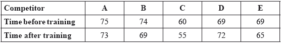
Apply an appropriate test at the 1% significance level to decide whether the training schedule improves competitors’ times, stating clearly the null and alternative hypotheses. (It may be assumed that the distributions of the times before and after training are normal.)
Markscheme
\({{\text{H}}_0}\): the training schedule does not help improve times (or \(\mu = 0\)) A1
\({{\text{H}}_1}\): the training schedule does help improve times (or \(\mu > 0\)) A1
Note: Subsequent marks can be awarded even if the hypotheses are not stated.
(Assuming difference of times is normally distributed.)
let \(d{\text{ time before training }}-{\text{ time after training}}\) (M1)
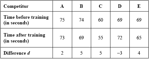
EITHER
\(n = 5,{\text{ }}\sum {d = 13,{\text{ }}} \sum {{d^2} = 79 \Rightarrow s_{n - 1}^2 = \frac{1}{4}\left( {79 - \frac{{169}}{5}} \right) = 11.3} \) (M1)
(small sample) so use a one-sided t-test (M1)
Note: The “one-sided” t-test may have been seen above when stating \({{\text{H}}_1}\).
\(t = \frac{{2.6}}{{\sqrt {\frac{{11.3}}{5}} }} = 1.7 \ldots \) A1
\(v = 4\), A1
at the 1% level the critical value is 3.7 A1
since \({\text{3.7}} > {\text{1.7}} \ldots \)
\({{\text{H}}_0}\) is accepted (insufficient evidence to reject \({{\text{H}}_0}\)) R1
Note: Follow through their t-value.
OR
(small sample) so use a one-sided t-test (M1)
\(p = 0.079 \ldots \) A4
since \(0.079 \ldots > 0.01\)
\({{\text{H}}_0}\) is accepted (insufficient evidence to reject \({{\text{H}}_0}\)) R1
Note: Follow through their p-value.
Note: Accept \(d = {\text{time after training }}-{\text{ time before training throughout}}\).
[10 marks]
Examiners report
It was again disappointing to see many candidates giving incorrect hypotheses. A common error was to give the hypotheses the wrong way around. Candidates should be aware that in this type of problem the null hypothesis always represents the status quo. Also, some candidates defined ‘\(d = {\text{time before }}-{\text{ time after}}\)’ and then gave the hypotheses incorrectly as \({{\text{H}}_0}:d = 0\) or \(\bar d = 0;{\text{ }}{{\text{H}}_1}:d > 0\) or \(\bar d > 0\). It is important to note that the parameter being tested here is \(E(d)\) or \({\mu _d}\) although \(\mu \) was accepted.
A population is known to have a normal distribution with a variance of 3 and an unknown mean \(\mu \) . It is proposed to test the hypotheses \({{\text{H}}_0}:\mu = 13,{\text{ }}{{\text{H}}_1}:\mu > 13\) using the mean of a sample of size 2.
(a) Find the appropriate critical regions corresponding to a significance level of
(i) 0.05;
(ii) 0.01.
(b) Given that the true population mean is 15.2, calculate the probability of making a Type II error when the level of significance is
(i) 0.05;
(ii) 0.01.
(c) How is the change in the probability of a Type I error related to the change in the probability of a Type II error?
Markscheme
(a) With \({{\text{H}}_0},{\text{ }}\bar X \sim {\text{N}}\left( {13,\frac{3}{2}} \right) = {\text{N(13, 1.5)}}\) (M1)(A1)
(i) 5 % for N(0,1) is 1.645
so \(\frac{{\bar x - 13}}{{\sqrt {1.5} }} = 1.645\) (M1)(A1)
\(\bar x = 13 + 1.645\sqrt {1.5} \)
\( = 15.0\,\,\,\,\,{\text{(3 s.f.)}}\) A1 N0
\({\text{[15.0, }}\infty {\text{[}}\)
(ii) 1% for N(0, 1) is 2.326
so \(\frac{{\bar x - 13}}{{\sqrt {1.5} }} = 2.326\) (M1)(A1)
\(\bar x = 13 + 2.326\sqrt {1.5} \)
\( = 15.8\,\,\,\,\,{\text{(3 s.f., accept 15.9)}}\) A1 N0
\({\text{[15.8, }}\infty {\text{[}}\)
[8 marks]
(b) (i) \(\beta = {\text{P}}(\bar X < 15.0147)\) M1
\( = 0.440\) A2
(ii) \(\beta = {\text{P}}(\bar X < 15.8488)\) M1
\( = 0.702\) A2
[6 marks]
(c) The probability of a Type II error increases when the probability of a Type I error decreases. R2
[2 marks]
Total [16 marks]
Examiners report
This question proved to be the most difficult. The range of solutions ranged from very good to very poor. Many students thought that \(P(TypeI) = 1 - P(TypeII)\) when in fact \(1 - P(TypeII)\) is the power of the test.
Eric plays a game at a fairground in which he throws darts at a target. Each time he throws a dart, the probability of hitting the target is \(0.2\). He is allowed to throw as many darts as he likes, but it costs him \($1\) a throw. If he hits the target a total of three times he wins \($10\).
Find the probability he has his third success of hitting the target on his sixth throw.
(i) Find the expected number of throws required for Eric to hit the target three times.
(ii) Write down his expected profit or loss if he plays until he wins the \($10\).
If he has just \($8\), find the probability he will lose all his money before he hits the target three times.
Markscheme
METHOD 1
let \(X\) be the number of throws until Eric hits the target three times
\(X \sim {\text{NB(3, 0.2)}}\) (M1)
\({\text{P}}(X = 6) = \left( {\begin{array}{*{20}{c}} 5 \\ 2 \end{array}} \right){0.8^3} \times {0.2^3}\) (A1)
\( = 0.04096\;\;\;\left( { = \frac{{128}}{{3125}}} \right)\;\;\;\)(exact) A1
METHOD 2
let \(X\) be the number of hits in five throws
\(X\) is \({\text{B}}(5,{\text{ }}0.2)\) (M1)
\({\text{P}}(X = 2) = \left( {\begin{array}{*{20}{c}} 5 \\ 2 \end{array}} \right){0.2^2} \times {0.8^3}\;\;\;(0.2048)\) (A1)
\(P\)(3rd hit on 6th throw) \( = \left( {\begin{array}{*{20}{c}} 5 \\ 2 \end{array}} \right){0.2^2} \times {0.8^3} \times 0.2 = 0.04096\left( { = \frac{{128}}{{3125}}} \right)\;\;\;\)(exact) A1
[3 marks]
(i) \({\text{expected number of throws}} = \frac{3}{{0.2}} = 15\) (M1)A1
(ii) \({\text{profit}} = (10 - 15) = - \$ 5{\text{ or loss}} = \$ 5\) A1
[3 marks]
METHOD 1
let \(Y\) be the number of times the target is hit in \(8\) throws
\(Y \sim {\text{B}}(8,{\text{ }}0.2)\) (M1)
\({\text{P}}(Y \le 2)\) (M1)
\( = 0.797\) A1
METHOD 2
let the \({3^{{\text{rd}}}}\) hit occur on the \({Y^{{\text{th}}}}\) throw
\(Y{\text{ is NB}}(3,{\text{ }}0.2)\) (M1)
\({\text{P}}(Y > 8) = 1 - {\text{P}}(Y \le 8)\) (M1)
\( = 0.797\) A1
[3 marks]
Total [9 marks]
Examiners report
Part (a) was well answered, using the negative binomial distribution \(NB(3,{\text{ }}0.2)\), by many candidates. Some candidates began by using the binomial distribution \(B(5,{\text{ }}0.2)\) which is a valid method as long as it is followed by multiplying by 0.2 but this final step was not always carried out successfully.
Part (b) was well answered by the majority of candidates.
In (c), candidates who used the binomial distribution \(B(8,{\text{ }}0.2)\) were generally successful. Candidates who used the negative binomial distribution \(Y \approx NB(3,{\text{ }}0.2)\) to evaluate \(P(Y > 8)\) were usually unsuccessful because of the large amount of computation involved.
A teacher wants to determine whether practice sessions improve the ability to memorize digits.
He tests a group of 12 children to discover how many digits of a twelve-digit number could be repeated from memory after hearing them once. He gives them test 1, and following a series of practice sessions, he gives them test 2 one week later. The results are shown in the table below.

(a) State appropriate null and alternative hypotheses.
(b) Test at the 5 % significance level whether or not practice sessions improve ability to memorize digits, justifying your choice of test.
Markscheme
(a) \({{\text{H}}_0}:d = 0;{\text{ }}{{\text{H}}_1}:d > 0\), where d is the difference in the number of digits remembered A1A1
[2 marks]
(b) A2
A2
Notes: Award A2 for the correct d values.
Award A1 for one error, A0 for two or more errors.
Use the t-test because the variance is not known M1R1
By GDC
t = 2.106… (A2)
EITHER
p-value = 0.0295 (accept any value that rounds to this number) A2
Since 0.0295 < 0.05 there is evidence that practice sessions improve ability to memorize digits R1
OR
The critical value of t is 1.796 A2
Since 2.106... > 1.796 there is evidence that practice sessions improve ability to memorize digits R1
Note: Award M1R1A1A1R1 for testing equality of means (t = –1.46, p-value = 0.08) .
[9 marks]
Total [11 marks]
Examiners report
Although this question was reasonably well done the hypotheses were often not stated precisely and the fact that the two data sets were dependent escaped many candidates.
The continuous random variable X has probability density function f given by
\[f(x) = \left\{ {\begin{array}{*{20}{c}}
{2x,}&{0 \leqslant x \leqslant 0.5,} \\
{\frac{4}{3} - \frac{2}{3}x,}&{0.5 \leqslant x \leqslant 2} \\
{0,}&{{\text{otherwise}}{\text{.}}}
\end{array}} \right.\]
Sketch the function f and show that the lower quartile is 0.5.
(i) Determine E(X ).
(ii) Determine \({\text{E}}({X^2})\).
Two independent observations are made from X and the values are added.
The resulting random variable is denoted Y .
(i) Determine \({\text{E}}(Y - 2X)\) .
(ii) Determine \({\text{Var}}\,(Y - 2X)\).
(i) Find the cumulative distribution function for X .
(ii) Hence, or otherwise, find the median of the distribution.
Markscheme
piecewise linear graph

correct shape A1
with vertices (0, 0), (0.5, 1) and (2, 0) A1
LQ: x = 0.5 , because the area of the triangle is 0.25 R1
[3 marks]
(i) \({\text{E}}(X) = \int_0^{0.5} {x \times 2x{\text{d}}x + \int_{0.5}^2 {x \times \left( {\frac{4}{3} - \frac{2}{3}x} \right){\text{d}}x = \frac{5}{6}{\text{ }}( = 0.833...)} } \) (M1)A1
(ii) \({\text{E}}({X^2}) = \int_0^{0.5} {{x^2} \times 2x{\text{d}}x + \int_{0.5}^2 {{x^2} \times \left( {\frac{4}{3} - \frac{2}{3}x} \right){\text{d}}x = \frac{7}{8}{\text{ }}( = 0.875)} } \) (M1)A1
[4 marks]
(i) \({\text{E}}(Y - 2X) = 2{\text{E}}(X) - 2{\text{E}}(X) = 0\) A1
(ii) \({\text{Var}}\,(X) = \left( {{\text{E}}({X^2}) - {\text{E}}{{(X)}^2}} \right) = \frac{{13}}{{72}}\) A1
\(Y = {X_1} + {X_2} \Rightarrow {\text{Var}}\,(Y) = 2{\text{Var }}(X)\) (M1)
\({\text{Var}}\,(Y - 2X) = 2{\text{Var}}\,(X) + 4{\text{Var}}\,(X) = \frac{{13}}{{12}}\) M1A1
[5 marks]
(i) attempt to use \(cf(x) = \int {f(u){\text{d}}u} \) M1
obtain \(cf(x) = \left\{ {\begin{array}{*{20}{c}}
{{x^2},}&{0 \leqslant x \leqslant 0.5,} \\
{\frac{{4x}}{3} - \frac{1}{3}{x^2} - \frac{1}{3},}&{0.5 \leqslant x \leqslant 2,}
\end{array}} \right.\) \(\begin{array}{*{20}{c}}
{{\boldsymbol{A1}}} \\
{{\boldsymbol{A2}}}
\end{array}\)
(ii) attempt to solve \(cf(x) = 0.5\) M1
\(\frac{{4x}}{3} - \frac{1}{3}{x^2} - \frac{1}{3} = 0.5\) (A1)
obtain 0.775 A1
Note: Accept attempts in the form of an integral with upper limit the unknown median.
Note: Accept exact answer \(2 - \sqrt {1.5} \) .
[7 marks]
Examiners report
There was a curious issue about the lower quartile in part (a): The LQ coincides with a quarter of the range of the distribution \(\frac{2}{4} = 0.5\). Sadly this is wrong reasoning – the correct reasoning involves a consideration of areas.
There was a curious issue about the lower quartile in part (a): The LQ coincides with a quarter of the range of the distribution \(\frac{2}{4} = 0.5\). Sadly this is wrong reasoning – the correct reasoning involves a consideration of areas.
In part (b) many candidates used hand calculation rather than their GDC.
The random variable Y was not well understood, and that followed into incorrect calculations involving Y – 2X.
A random variable \(X\) has probability density function
\(f(x) = \left\{ {\begin{array}{*{20}{c}} 0&{x < 0} \\ {\frac{1}{2}}&{0 \le x < 1} \\ {\frac{1}{4}}&{1 \le x < 3} \\ 0&{x \ge 3} \end{array}} \right.\)
Sketch the graph of \(y = f(x)\).
Find the cumulative distribution function for \(X\).
Find the interquartile range for \(X\).
Markscheme
 A1
A1
Note: Ignore open / closed endpoints and vertical lines.
Note: Award A1 for a correct graph with scales on both axes and a clear indication of the relevant values.
[1 mark]
\(F(x) = \left\{ {\begin{array}{*{20}{c}} 0&{x < 0} \\ {\frac{x}{2}}&{0 \le x < 1} \\ {\frac{x}{4} + \frac{1}{4}}&{1 \le x < 3} \\ 1&{x \ge 3} \end{array}} \right.\)
considering the areas in their sketch or using integration (M1)
\(F(x) = 0,{\text{ }}x < 0,{\text{ }}F(x) = 1,{\text{ }}x \ge 3\) A1
\(F(x) = \frac{x}{2},{\text{ }}0 \le x < 1\) A1
\(F(x) = \frac{x}{4} + \frac{1}{4},{\text{ }}1 \le x < 3\) A1A1
Note: Accept \( < \) for \( \le \) in all places and also \( > \) for \( \ge \) first A1.
[5 marks]
\({Q_3} = 2,{\text{ }}{Q_1} = 0.5\) A1A1
\({\text{IQR is }}2 - 0.5 = 1.5\) A1
[3 marks]
Total [9 marks]
Examiners report
Part (a) was correctly answered by most candidates. Some graphs were difficult to mark because candidates drew their lines on top of the ruled lines in the answer book. Candidates should be advised not to do this. Candidates should also be aware that the command term ‘sketch’ requires relevant values to be indicated.
In (b), most candidates realised that the cumulative distribution function had to be found by integration but the limits were sometimes incorrect.
In (c), candidates who found the upper and lower quartiles correctly sometimes gave the interquartile range as \([0.5,{\text{ }}2]\). It is important for candidates to realise that that the word range has a different meaning in statistics compared with other branches of mathematics.